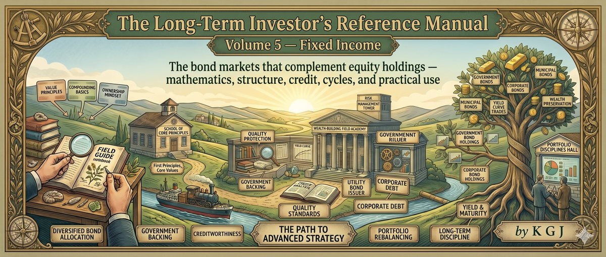
The Long-Term Investor's Reference Manual — Volume 5
Fixed Income The bond markets that complement equity holdings — mathematics, structure, credit, cycles, and practical use

Preface to Volume 5
Fixed income is the larger of the two major public asset classes. Global bond markets exceeded $135 trillion in 2024, against approximately $115 trillion in global equities. Despite this scale, fixed income receives substantially less attention from retail investors than equities, partly because bonds are more complex to analyse, partly because their structure is less intuitive than that of stocks, and partly because the popular financial press devotes far more coverage to equity markets.
This is a problem. Fixed income is a critical component of most balanced portfolios, particularly in distribution phase. The mathematics of bond pricing — duration, convexity, yield curves, credit spreads — are essential for understanding what bond holdings actually do. The behaviour of bonds across rate cycles, particularly the dramatic 2022 episode in which long-duration bonds fell more than 20%, illustrates why retail investors who treated bonds as "safe" without understanding the mechanics suffered substantial unexpected losses.
This volume is organised to support both the investor who will hold bonds primarily through ETFs and the investor who wants deeper engagement with bond markets. Sections 1 through 4 establish the foundations — what bonds are, the major categories, the mathematics of pricing, and the structure of yield curves. Sections 5 through 7 address credit analysis, the corporate bond market, and the behaviour of bonds in different environments. Sections 8 through 10 cover the practical implementation through ETFs and individual bonds, with attention to both United States and Australian context. Sections 11 and 12 address portfolio construction with bonds and the synthesis.
The mathematical content is denser than in previous volumes because it must be. Bond mathematics cannot be skipped if the investor is to understand what holdings do under different conditions. Worked examples are provided throughout. The investor who studies these slowly will emerge with capabilities that most retail investors lack and that produce meaningful advantages in portfolio construction and risk management.
A note on Australian context: the Australian fixed income market is structurally different from the United States market in several important ways. The corporate bond market is smaller and less accessible to retail investors. Hybrid securities (preference shares, capital notes, listed perpetual securities) play a larger role than in most other markets. Government and semi-government securities have specific characteristics that differ from US Treasuries and agencies. Where these differences matter, both contexts are addressed.
A second note on the relationship to equity investing covered in Volumes 3 and 4. Fixed income is not merely the residual after equity decisions. The choice of bond exposure — duration, credit quality, geographic and currency mix — is a substantive portfolio decision that affects total returns, volatility, and behaviour through cycles. Treating bonds as "the safe part of the portfolio" without engaging with what makes them safe (or not safe) under specific conditions is one of the more common retail investor errors.
Section 1 — What a Bond Actually Is
Before any analysis of bond markets, the working investor needs precise understanding of what a bond represents legally and economically. The popular framing — that bonds are loans that pay interest — is technically true but obscures features that matter substantially for analysis.
1.1 The legal structure of a bond
A bond is a debt instrument issued by a borrower (the issuer) to lenders (the bondholders), creating specific contractual obligations. The standard features:
Principal (also called face value or par value) is the amount the issuer promises to repay at maturity. The principal amount is fixed at issuance and does not change over the bond's life. Most bonds have a face value of $1,000 (in the United States) or A$1,000 to A$10,000 (in Australia), although institutional bonds can have much larger face values.
Coupon is the periodic interest payment the issuer makes to bondholders. Coupons are typically expressed as an annual percentage of face value and paid semi-annually (in the United States) or quarterly (more common in Australia and some other markets). A bond with a 5% coupon and $1,000 face value pays $50 per year, typically as $25 every six months.
Maturity is the date on which the issuer repays the principal. Bonds with maturities under one year are typically called money market instruments or short-term notes. Bonds with maturities of one to ten years are intermediate-term. Bonds with maturities greater than ten years are long-term. Some bonds have maturities of 30, 50, or 100 years; perpetual bonds have no fixed maturity at all.
Indenture is the legal document governing the bond, specifying all the terms of the contract. The indenture includes the coupon rate, payment dates, maturity, any provisions for early redemption (calls), restrictions on the issuer's behaviour (covenants), and other legal terms. The indenture is the controlling document for the bondholder's rights.
The contractual nature of bond obligations is critical. Unlike dividends on equity, which are discretionary and can be cancelled, coupon payments are contractual obligations. An issuer that fails to make a scheduled coupon payment is in default, with significant legal consequences. The discipline of contractual obligations is what makes bonds typically less risky than equity for the same issuer — bondholders have legal claims that equity holders do not.
1.2 Senior versus subordinated, secured versus unsecured
Within the broad category of debt, several gradations of priority exist:
Senior secured debt has the highest priority claim on the issuer's assets. The debt is secured by specific collateral (real estate, equipment, receivables) that bondholders can claim if the issuer defaults. Mortgages on real estate are the canonical example. In a default, senior secured creditors are paid first, often recovering most or all of their principal even when other creditors lose substantial amounts.
Senior unsecured debt has priority over subordinated debt but is not secured by specific collateral. The bondholders are general creditors of the issuer, with claims on whatever assets remain after secured creditors are paid. Most corporate bonds are senior unsecured.
Subordinated debt ranks below senior debt in priority. In a default, subordinated creditors are paid only after senior creditors are made whole. The lower priority is compensated by higher coupon rates.
Junior subordinated debt ranks below other subordinated debt, typically the lowest-priority debt instrument. In a default, junior subordinated creditors may receive little or nothing.
Hybrid securities sit between debt and equity, with features of both. Preference shares, capital notes, and various other hybrid instruments are common in some markets (particularly Australia, where they are major retail products). They typically have fixed coupon-like distributions but can be deferred under certain conditions, and they rank below all other debt in liquidation. Volume 5 covers hybrids in Section 9.
The ranking matters enormously in default scenarios. Recovery rates — the percentage of face value that creditors actually receive in a default — vary substantially by priority:
- Senior secured: typically 60-80% recovery historically
- Senior unsecured: typically 30-50% recovery
- Subordinated: typically 10-30% recovery
- Junior subordinated: typically 0-15% recovery
- Equity: typically 0% in formal default scenarios
These are averages with substantial variation. Specific defaults can produce very different outcomes depending on the issuer's specific financial position, the legal framework in the jurisdiction, and the negotiation dynamics in restructuring.
1.3 Fixed rate, floating rate, and inflation-linked
Bonds vary in how their coupon payments are determined:
Fixed rate bonds pay the same coupon throughout their life. The 5% coupon set at issuance remains 5% regardless of subsequent changes in market interest rates. The investor receives predictable nominal cash flows.
Floating rate bonds (also called variable rate bonds or floating rate notes) pay a coupon that resets periodically based on a reference rate. A typical structure: "3-month SOFR plus 1.5%" means the coupon resets every quarter to whatever the 3-month SOFR rate is at the reset date, plus 1.5 percentage points. As rates rise, the coupon rises; as rates fall, it falls. Floating rate bonds have less interest rate sensitivity than fixed rate bonds because the coupon adjusts.
Inflation-linked bonds have coupons or principal that adjust for inflation. Treasury Inflation-Protected Securities (TIPS) in the United States and inflation-linked gilts in the United Kingdom are major examples. The principal value adjusts upward with the consumer price index, and the coupon (typically a relatively low fixed rate) is paid on the inflation-adjusted principal. The investor receives real (inflation-adjusted) returns rather than nominal returns.
Step-up bonds have coupons that increase on a pre-specified schedule. Less common but used for specific purposes.
Zero-coupon bonds pay no coupons at all. Instead, they are issued at a discount to face value and redeemed at face value. The "interest" is the difference between issue price and face value. United States Treasury STRIPS are the most prominent zero-coupon government bonds.
The choice of structure matters for analysis. Fixed rate bonds have the highest interest rate sensitivity (covered in Section 3). Floating rate bonds have very low interest rate sensitivity but higher exposure to credit dynamics. Inflation-linked bonds have low real-rate sensitivity but high inflation breakeven sensitivity. Zero-coupon bonds have the highest interest rate sensitivity of any bond structure.
1.4 Callable, putable, and convertible features
Standard bonds have a fixed redemption schedule — coupon payments on specified dates and principal repayment at maturity. Some bonds have additional features that affect this schedule:
Callable bonds give the issuer the right to redeem the bond before maturity at a specified call price. The issuer typically calls the bond when interest rates have fallen substantially, allowing the issuer to refinance at lower rates. From the bondholder's perspective, callable bonds are unfavourable: the bondholder loses the high coupon when rates fall (the bond is called and proceeds must be reinvested at lower current rates) and keeps the bond when rates rise (when they would prefer to receive principal back to reinvest at higher current rates).
The asymmetric option granted to the issuer is compensated by higher coupons on callable bonds compared to equivalent non-callable bonds. The size of the call premium depends on the call structure (when it can be exercised, at what price) and on interest rate volatility.
Putable bonds give the bondholder the right to require the issuer to redeem the bond before maturity. The mirror image of callable bonds. Bondholders have an option that can be valuable if rates rise (allowing the bondholder to receive principal and reinvest at higher rates). The option is compensated by lower coupons on putable bonds. Putable bonds are less common than callable bonds.
Convertible bonds give the bondholder the right to convert the bond into a specified number of shares of the issuer's common stock. Convertible bonds combine features of debt (coupon payments, maturity, priority over equity) with features of equity (upside if the stock appreciates). The conversion option has value, which is reflected in lower coupons compared to equivalent non-convertible bonds. Convertible bonds are common in technology and high-growth sectors as financing for issuers and as equity-like investments with downside protection for buyers.
For long-term investors, the practical implications:
The presence of call features introduces uncertainty about actual cash flows and effective duration. Investors should be aware of call provisions and understand how the bond's performance differs from comparable non-callable bonds.
Convertible bonds are hybrid investments that should be evaluated as such — partly as bonds, partly as equity. Their behaviour depends on whether the underlying stock is significantly above, near, or below the conversion price.
For most retail investors, focusing on standard non-callable, non-convertible bonds keeps the analysis simpler and avoids the complications of optionality.
1.5 The cash flow profile of a typical bond
Putting these elements together, the cash flow profile of a typical fixed-rate bond can be illustrated:
Consider a $1,000 face value bond with a 5% annual coupon (paid as $25 semi-annually), maturing in 10 years.
The cash flows from the bondholder's perspective:
- At purchase: pay the market price (which may differ from face value)
- Every six months for 10 years: receive $25 coupon payment
- At maturity: receive $1,000 principal repayment
Total payments received: 20 coupons of $25 ($500 total) plus $1,000 principal = $1,500
Total return depends on the purchase price and any reinvestment of coupons. If purchased at face value, the holder receives a current yield of 5% (50/1000) and a yield to maturity of 5%. If purchased at a premium (say $1,050) the yield to maturity is below 5% because the holder pays $1,050 today to receive $1,500 over 10 years; the implicit annual return is lower than 5%. If purchased at a discount (say $950), the yield to maturity is above 5%.
This relationship between price and yield is the foundation of bond mathematics, covered in detail in Section 3.
1.6 Why investors hold bonds
Bonds serve several specific functions in investor portfolios:
Income generation. Coupon payments provide predictable cash flow that can be used to fund living expenses, particularly important in retirement. The reliability of coupon payments (subject to credit risk) makes bonds suitable for income-focused strategies.
Capital preservation. High-quality short-duration bonds preserve capital with low volatility. They are appropriate for funds that may need to be accessed within a few years.
Portfolio diversification. Bonds typically have lower correlation with equities than equities have with each other, so adding bonds to an equity portfolio reduces overall volatility. The diversification benefit varies across regimes — bonds and equities can move in the same direction (both falling) during inflation shocks, as 2022 demonstrated.
Defensive positioning. In severe equity downturns, high-quality long-duration government bonds historically appreciate as investors flee to safety and as central banks ease monetary policy. The 2008-2009 crisis produced strong positive returns for long government bonds even as equities crashed.
Liability matching. Investors with specific known future obligations (pension payments, insurance claims, scheduled expenses) can match bond cash flows to those obligations, eliminating timing risk. This is the foundational use of bonds for institutional investors but applies in modified form to retail investors as well.
Portfolio rebalancing. Bond holdings provide a source of capital for rebalancing during equity market declines. Investors who hold bonds and maintain discipline can buy equities at reduced prices using bond proceeds, capturing some of the rebound when markets recover.
The relative weight of these functions depends on the investor's circumstances. A young accumulator may hold few bonds because none of these functions are particularly important to them. A retiree may hold substantial bonds because income generation, capital preservation, and liability matching are central to their situation. The appropriate bond allocation is therefore highly individual.
1.7 What bonds do not provide
A balanced treatment requires acknowledging what bonds do not provide:
Inflation protection. Standard fixed-rate bonds lose real value during inflation. The 2022 episode reminded investors of this — bonds that yielded 2-3% nominal in environments where inflation reached 9% produced large real losses. Inflation-linked bonds address this directly but at the cost of lower yields and added complexity.
Long-term wealth building. Over very long horizons, equities have substantially outperformed bonds in nominal and real terms. A portfolio that is heavily weighted toward bonds during accumulation phase will produce lower terminal wealth than a more equity-heavy portfolio, despite the higher volatility. The trade-off between volatility reduction and return reduction is real.
Immunity from rate cycles. The 2022 rate cycle produced dramatic losses in long-duration bond holdings. The Bloomberg US Aggregate Bond Index lost approximately 13% in 2022 — its worst year in decades. Long-duration government bond ETFs (like TLT) lost over 30%. Investors who held bonds expecting them to be the "safe" portion of their portfolios were surprised. Bonds are not safe in any absolute sense; they are safer than equities under specific conditions but vulnerable to other conditions.
Protection against issuer-specific risks. Corporate bonds, municipal bonds, and emerging market bonds carry credit risk that government bonds do not. Even within these categories, individual issuers can default and produce permanent capital loss. Diversification helps but does not eliminate these risks.
Liquidity during stress. Some bond market segments become illiquid during stress periods. Corporate bonds, municipal bonds, and emerging market bonds can become very difficult to sell at reasonable prices during severe market dislocations. Even high-quality bonds saw spreads widen substantially during the 2008 and March 2020 episodes.
The honest framing: bonds have specific and valuable roles in portfolios, but they are not the universal "safe" asset that retail investors sometimes assume. The role of bonds depends on the specific bonds chosen and the conditions under which they are held.
Section 2 — The Taxonomy of Fixed Income
The fixed income universe is much broader than the equity universe. This section maps the major categories with attention to their specific characteristics, risks, and roles.
2.1 Government bonds
Government bonds are debt obligations of national governments. They are typically the largest single category of fixed income securities and serve as the benchmark for the broader market.
United States Treasuries are the most important government bond market globally. The US Treasury issues several specific types:
Treasury bills (T-bills) have maturities of 4, 8, 13, 17, 26, or 52 weeks. They are zero-coupon instruments — issued at a discount to face value and redeemed at face value. They are the most liquid fixed-income instruments globally and serve as the primary risk-free reference for short-term financial markets.
Treasury notes have maturities of 2, 3, 5, 7, or 10 years. They pay semi-annual coupons. The 10-year note is particularly important as a benchmark for longer-term interest rates and as a reference for mortgage rates.
Treasury bonds have maturities of 20 or 30 years. They pay semi-annual coupons. The 30-year bond is the longest maturity routinely issued.
Treasury Inflation-Protected Securities (TIPS) have inflation-adjusted principal. Maturities range from 5 to 30 years.
Treasury Floating Rate Notes (FRNs) have rates that reset based on the 13-week T-bill rate. Maturities are 2 years.
US Treasuries are considered effectively risk-free for credit purposes — the US government can always print dollars to pay dollar-denominated obligations, even if the resulting inflation produces real losses. The "risk-free" designation refers to nominal default risk, not real economic risk.
Australian Commonwealth Government Securities (CGS) are the equivalent in Australia. The Australian Office of Financial Management issues:
Treasury bonds with maturities ranging from 2 to 30 years, paying semi-annual coupons.
Treasury indexed bonds with inflation-adjusted principal, similar to US TIPS.
Treasury notes with shorter maturities, typically 1 to 6 months, used for cash management.
The Australian government bond market is much smaller than the US market — total CGS outstanding is approximately A$900 billion versus over US$25 trillion in US Treasuries. This affects liquidity and the depth of derivative markets built on the underlying bonds.
Other developed market sovereigns include UK Gilts, German Bunds, Japanese Government Bonds (JGBs), Canadian Government Bonds, and various others. These are typically high-quality but with specific characteristics:
UK Gilts include both conventional bonds and index-linked gilts. The UK has issued some very long-duration bonds (50-year and 100-year maturities exist, though most are 30 years or shorter).
German Bunds serve as the European benchmark. The 10-year Bund is the reference rate for European fixed income markets, similar to the role of the 10-year Treasury in US markets.
Japanese Government Bonds have unusual characteristics due to Japan's long experience with very low (and sometimes negative) interest rates. The Bank of Japan's yield curve control policy has shaped JGB yields directly. JGBs are the largest bond market outside the US.
Emerging market sovereigns are debt issued by developing-economy governments. They typically offer higher yields than developed-market sovereigns but carry substantially higher credit risk. Major issuers include Brazil, Mexico, Russia (now mostly inaccessible to Western investors after 2022 sanctions), South Africa, Turkey, India, Indonesia, and various others.
Emerging market sovereign debt comes in two main flavours:
Hard currency debt is denominated in major reserve currencies (typically US dollars, sometimes euros). The issuer bears the currency risk; the bondholder bears credit risk only. Hard currency emerging market bonds are popular with international investors.
Local currency debt is denominated in the issuer's domestic currency. The bondholder bears both credit risk and currency risk. Yields are typically higher than hard currency equivalents to compensate for the additional risk.
2.2 Government agency and supranational bonds
Several quasi-government issuers occupy a space between sovereign and corporate:
US agency debt is issued by federal agencies and government-sponsored enterprises:
Federal agencies such as Ginnie Mae have full faith and credit backing of the US government, equivalent to Treasury debt for credit purposes.
Government-sponsored enterprises (GSEs) including Fannie Mae, Freddie Mac, and the Federal Home Loan Banks have implicit but not explicit US government backing. Their debt typically trades at small spreads to Treasuries reflecting the implicit guarantee.
Mortgage-backed securities (MBS) issued by Fannie Mae, Freddie Mac, and Ginnie Mae represent pooled mortgages. These are a major asset class in their own right, covered separately below.
Australian semi-government bonds are debt issued by Australian state governments. Major issuers include New South Wales Treasury Corporation (NSW T-Corp), Victorian Funding Authority (VFA), Queensland Treasury Corporation (QTC), and Western Australian Treasury Corporation (WATC). These are sometimes called "semis" in market shorthand.
Semi-government bonds typically yield 20-50 basis points above Commonwealth Government Securities, reflecting their slightly higher credit risk (state governments cannot print currency, although they have substantial revenue powers and historical Commonwealth support). For Australian retail investors, semis are a useful intermediate between Commonwealth bonds and corporate debt.
Supranational bonds are issued by international organisations including the World Bank, European Investment Bank, Inter-American Development Bank, Asian Development Bank, and various others. These typically carry very high credit ratings (often AAA) reflecting strong shareholder support from member governments. They yield slightly more than equivalent sovereign debt.
2.3 Municipal bonds
Municipal bonds (munis) are debt issued by state and local governments and their agencies. They are a major asset class in the United States, with approximately $4 trillion outstanding.
The defining feature of US municipal bonds is their tax treatment. Interest on most municipal bonds is exempt from US federal income tax, and often from state income tax for residents of the issuing state. This produces a yield differential between munis and taxable bonds — munis can yield substantially less than equivalent taxable bonds while still providing equivalent or better after-tax returns to investors in higher tax brackets.
The two major categories of US municipal bonds:
General obligation (GO) bonds are backed by the issuer's general taxing power. The issuer pledges to use whatever resources are necessary, including raising taxes if needed, to make payments. GO bonds from financially strong municipalities are very high quality.
Revenue bonds are backed by specific revenue streams from particular projects — toll roads, water systems, hospitals, airports, and various other facilities. The bonds are repaid from the revenues of the underlying project, not from general municipal funds. Revenue bonds vary widely in quality depending on the underlying project's economics.
US municipal bonds have historically been considered very safe, but defaults do occur. Detroit's 2013 bankruptcy, Puerto Rico's 2017 bankruptcy, and various smaller municipal defaults have demonstrated that munis are not free of credit risk. The Detroit case in particular involved substantial losses for some categories of municipal bondholders.
For Australian investors, US municipal bonds are not particularly relevant — the tax exemption applies only to US federal taxes, providing no benefit to non-US investors. Australia has a very small municipal bond market (state government semi-government bonds are different and covered above), so the asset class is essentially absent from Australian portfolios.
2.4 Corporate bonds
Corporate bonds are debt issued by companies. The corporate bond universe is enormous and varied — from very high-quality investment grade debt issued by major multinationals to highly speculative high yield debt from distressed issuers.
The credit rating system divides corporate bonds into broad categories:
Investment grade bonds are rated BBB- and above by S&P (or Baa3 and above by Moody's). These are bonds with relatively low default risk, suitable for institutional investors with conservative mandates. The investment grade universe is further divided:
AAA/Aaa: highest quality, minimal default risk. Very few corporate issuers are rated AAA — typically only a handful at any time. Microsoft and Johnson & Johnson have historically been among them.
AA/Aa: very high quality, low default risk. Major banks, oil majors, and similar large stable issuers.
A: high quality, low but not minimal default risk. Many large multinational corporations.
BBB/Baa: medium-grade quality, moderate default risk. The largest single category of investment grade debt.
High yield bonds (also called speculative grade or "junk" bonds) are rated below investment grade. These carry substantially higher default risk but offer correspondingly higher yields. Categories:
BB/Ba: below investment grade but with reasonable financial profile. Some "fallen angels" — companies that were investment grade but were downgraded — populate this category.
B: speculative quality with meaningful default risk.
CCC/Caa and below: substantial default risk. Many bonds in these categories are trading at deep discounts reflecting market expectations of restructuring or default.
The boundary between investment grade and high yield (BBB- versus BB+) is structurally important because many institutional investors have mandates restricting their investments to investment grade. A downgrade across this boundary can produce forced selling and substantial price declines.
The mathematics of credit ratings and default rates are covered in Section 5. The key points for now:
Investment grade corporate bonds historically have very low default rates, typically under 1% per year cumulative for the strongest categories.
High yield bonds have higher default rates, varying with the credit cycle. Through-the-cycle averages are 4-5% per year for the high yield universe overall, with substantial variation across rating categories.
Corporate bond yields decompose into a risk-free component (the equivalent Treasury yield) plus a credit spread (compensation for default risk and other factors). The credit spread component varies substantially over time and across issuers.
2.5 Securitised products
Securitised products are bonds backed by pools of underlying assets. The pool is typically held in a special purpose vehicle that issues the bonds, providing structural separation from the assets' originator.
Mortgage-backed securities (MBS) are backed by pools of residential mortgages. The major categories:
Agency MBS are issued by Fannie Mae, Freddie Mac, and Ginnie Mae and represent pools of conforming mortgages (those meeting agency standards on size, credit quality, and other criteria). Agency MBS carry implicit (Fannie/Freddie) or explicit (Ginnie Mae) US government backing, making them very high credit quality. The main risk is prepayment risk — when interest rates fall, homeowners refinance and prepay mortgages, returning principal to MBS holders earlier than expected (forcing reinvestment at lower current rates).
Non-agency MBS are issued by private institutions and represent pools of mortgages that don't conform to agency standards (jumbo loans, alt-A loans, subprime loans). These have full credit risk and were at the center of the 2008 financial crisis.
Asset-backed securities (ABS) are backed by pools of non-mortgage assets including auto loans, credit card receivables, student loans, equipment leases, and various other categories. ABS are smaller than MBS in total outstanding but represent a meaningful share of the fixed income market.
Collateralised loan obligations (CLOs) are securitisations of corporate loans, typically leveraged loans (loans to below-investment-grade companies). CLOs have grown dramatically since the 2008 crisis and now represent a major segment of structured credit. They have specific structural features (subordination tranches, overcollateralisation, interest rate hedging) that affect their risk profile.
Collateralised debt obligations (CDOs) in the broader sense include CLOs but also include securitisations of other debt instruments. CDOs of MBS were major contributors to the 2008 crisis. Modern CDOs are typically more conservatively structured but the asset class retains some reputational concerns.
For most retail investors, direct exposure to securitised products is limited. They are typically accessed through diversified bond ETFs (which include them as part of the overall index exposure) rather than through specific securitised products.
2.6 International bonds
International bonds — debt issued by foreign sovereigns or corporations in foreign currencies — add geographic and currency dimensions to the basic credit analysis.
The major considerations:
Currency exposure. As discussed in Volume 2, foreign-currency bonds combine bond returns with currency returns. The combined return can be substantially different from the local return, making unhedged foreign bonds essentially currency speculations with bond yields.
Hedging considerations. Most institutional foreign bond holdings are currency-hedged through forward contracts or similar instruments. Currency hedging eliminates the currency exposure but introduces hedging costs that vary by currency pair and rate environment. In normal markets, hedging costs for major currency pairs are small (a few basis points per year). In stress periods, hedging costs can rise substantially.
Sovereign credit considerations. Foreign sovereign bonds carry the credit risk of the issuing government. For developed-market sovereigns, this is typically very low. For emerging-market sovereigns, it is substantially higher.
Tax and regulatory considerations. International bonds may be subject to withholding taxes on coupon payments, with treaty-based reductions for some investor types. Tax treaty considerations can produce material differences in after-tax returns.
For Australian investors, international bond exposure is typically obtained through globally-diversified bond ETFs or through Australian-domiciled funds that hold international debt with currency hedging. Direct holding of individual international bonds is uncommon for retail investors due to the complexity and minimum size requirements.
2.7 Other fixed income categories
Several smaller but important categories complete the fixed income universe:
Convertible bonds were mentioned in Section 1. They occupy a hybrid space between debt and equity. Convertible-specific ETFs and mutual funds exist.
Hybrid securities including preference shares, capital notes, and listed perpetual securities are particularly important in Australian retail markets. These typically pay higher distributions than ordinary debt but with various features (deferral options, conversion conditions, optional redemption) that complicate analysis. Section 9 addresses hybrids in detail.
Bank loans (also called leveraged loans) are non-public debt instruments held primarily by institutional investors. They are typically floating rate, secured by company assets, and subordinated to traditional senior debt only in specific circumstances. CLO structures aggregate bank loans into investable products, making them accessible to broader investor bases.
Catastrophe bonds are structured securities that pay coupons unless specified catastrophic events occur (major hurricanes, earthquakes, etc.). They have low correlation with other fixed income but very specific risk characteristics. They are primarily institutional investments.
Distressed debt is debt of companies in or near default, often trading at substantial discounts. This is a specialised area requiring legal and operational expertise to navigate the bankruptcy process. It is institutional rather than retail.
2.8 The Australian fixed income universe in particular
For Australian retail investors, the practical investable universe is more limited than the US equivalent:
Commonwealth Government Securities are accessible through ETFs or direct purchases. Direct purchases require a relatively large minimum (usually A$10,000 or more per holding) and are typically done through brokers.
Semi-government bonds are similar to CGS but with slightly higher yields. Available through ETFs or direct purchases through specialist brokers.
Australian corporate bonds are a smaller market than the US equivalent and have limited retail accessibility. Most corporate bonds in Australia are issued in institutional sizes and through over-the-counter markets that are difficult for retail investors to access. Some corporate bonds list on the ASX as "exchange-traded bonds" but the universe is small.
Hybrid securities (covered in detail in Section 9) are the most accessible "fixed income alternative" for Australian retail investors, with substantial volumes of listed hybrids available on the ASX. However, hybrids are not pure fixed income — they have equity-like features that change their risk profile.
International fixed income through Australian-domiciled ETFs provides access to global bond markets. These are typically currency-hedged to AUD. Examples include VIF (Vanguard International Fixed Income Index), VBND (Vanguard Diversified Bond Index), and various others.
Term deposits are not bonds in the strict sense but serve similar income-and-capital-preservation functions for Australian retail investors. They are bank obligations rather than bonds, but the cash flow profile is analogous. Major banks offer term deposits with maturities from 1 month to 5 years, with rates that vary with the broader yield curve.
The practical implication for Australian retail investors is that fixed income exposure typically comes through:
- Bond ETFs (covering CGS, semis, corporate, international)
- Hybrid securities (with appropriate caution about their equity-like features)
- Term deposits and cash products
- Inside superannuation, where the trustee may hold a wider range of fixed income directly
This is a more constrained universe than US retail investors face, but it is sufficient for most portfolio purposes. The key is to match the ETF or product to the desired exposure (duration, credit quality, currency hedging) rather than to attempt direct corporate bond investing that retail Australians have limited access to anyway.
Section 3 — The Mathematics of Bond Pricing
The mathematics of bond pricing are the foundation for understanding what bond holdings actually do. The relationships between yield, price, duration, and convexity govern bond behaviour across all conditions. This section develops the mathematics with worked examples and explicit attention to practical implications.
3.1 Present value of bond cash flows
A bond's price is the present value of its expected cash flows, discounted at an appropriate yield. The general formula:
Price = Σ [Coupon / (1 + y)^t] + [Face Value / (1 + y)^N]
Where:
- Coupon is the periodic coupon payment
- y is the yield per period
- t is the time of each cash flow
- N is the number of periods until maturity
For a bond with annual coupon payments, this is straightforward. For a bond with semi-annual coupon payments (most common in US Treasuries and corporates), the formula uses semi-annual periods and the per-period yield is half the annualised yield-to-maturity.
A worked example. Consider a 10-year Treasury bond with $1,000 face value, 5% annual coupon paid semi-annually ($25 every six months), and a market yield to maturity of 4%.
Number of periods: 20 (semi-annual) Per-period yield: 2% (4% / 2) Per-period coupon: $25
Price = Σ [$25 / (1.02)^t] for t = 1 to 20 + [$1,000 / (1.02)^20]
Calculating:
- Sum of present values of coupons: $25 × [1 - (1.02)^(-20)] / 0.02 = $25 × 16.3514 = $408.78
- Present value of face value: $1,000 / (1.02)^20 = $1,000 / 1.4859 = $672.97
- Total price: $408.78 + $672.97 = $1,081.75
A bond with a 5% coupon priced to yield 4% trades at a premium ($1,081.75 versus $1,000 face value) because the coupon exceeds the market yield. The investor pays $81.75 above face value to receive the higher-than-market coupon over the bond's life.
The same bond at a 5% market yield would trade at par ($1,000), and at a 6% market yield would trade at a discount (approximately $925.61 by the same calculation).
This relationship — bonds trading at premiums when their coupons exceed market yields, at par when coupons equal market yields, and at discounts when coupons are below market yields — is the foundation of bond pricing.
3.2 Yield to maturity
Yield to maturity (YTM) is the discount rate that makes the present value of a bond's cash flows equal to its current price. It is the rate of return an investor would earn if they bought the bond at the current price, held it to maturity, received all coupons, and reinvested them at the YTM rate.
YTM is found by solving the bond pricing formula for y, given the price:
Price = Σ [Coupon / (1 + y)^t] + [Face Value / (1 + y)^N]
This requires iterative calculation; there is no closed-form solution. In practice, YTM is calculated by spreadsheet functions (Excel's YIELD function), bond calculator software, or financial APIs.
The YTM has specific assumptions that should be understood:
Hold to maturity. YTM assumes the bond is held until it matures. If sold earlier, the actual return depends on the price at sale, which depends on prevailing yields at that time.
Coupons reinvested at YTM. YTM assumes that all coupon payments are reinvested at the same YTM rate. This is unrealistic — actual reinvestment rates vary as market rates change. The reinvestment rate assumption can produce substantial differences between calculated YTM and actual realised returns.
No defaults. YTM assumes the issuer makes all promised payments. For high-quality government bonds this is reasonable; for corporate or emerging market bonds, expected returns adjusted for default probability differ from YTM.
No taxes or transaction costs. YTM is a gross figure that does not account for taxation of coupons or capital gains, or for transaction costs on purchase or sale.
For practical bond evaluation, YTM is the single most important number. It tells the investor what return they can expect under the assumed conditions. Higher YTM means higher expected return, all else being equal. The comparison of YTMs across bonds (adjusted for credit, duration, and other characteristics) is the core of relative value analysis in fixed income.
3.3 Current yield versus yield to maturity
A common confusion is between current yield and yield to maturity. These are related but different concepts.
Current yield is the annual coupon divided by the current price:
Current Yield = Annual Coupon / Current Price
For our 5% coupon bond priced at $1,081.75, the current yield is $50 / $1,081.75 = 4.62%.
Yield to maturity is 4% (the discount rate that gives the price of $1,081.75).
The two yields differ because YTM accounts for the capital loss the holder will experience as the bond's price approaches face value at maturity. The bond purchased at $1,081.75 will be worth $1,000 at maturity — a capital loss of $81.75. This loss is amortised over the bond's life and reduces the yield from the current yield level (4.62%) to the YTM (4.00%).
For bonds trading at a premium, YTM is below current yield (the capital loss reduces the return). For bonds trading at a discount, YTM is above current yield (the capital gain at maturity adds to the return). For bonds trading at par, YTM equals current yield equals the coupon rate.
For practical bond evaluation, YTM is the relevant measure. Current yield can be misleading because it ignores the capital gain or loss component.
3.4 Duration: the foundational concept
Duration is the most important single concept in bond mathematics after yield. It measures the bond's sensitivity to changes in interest rates.
The intuitive definition: duration is the weighted average time to receive the bond's cash flows, where the weights are the present values of those cash flows.
The mathematical definition (Macaulay duration):
Duration = Σ [t × PV(CF_t)] / Price
Where PV(CF_t) is the present value of the cash flow at time t.
For our 10-year, 5% coupon bond yielding 4% (priced at $1,081.75), the duration is approximately 7.8 years. Each cash flow contributes to duration weighted by its present value:
- The first coupon (at year 0.5) has a large weight due to its proximity in time, but small dollar weight in the calculation.
- The principal payment (at year 10) has a smaller weight in the calculation due to discounting, but contributes substantially because it is the largest cash flow.
- The intermediate coupons contribute proportionally based on their time and present value.
The weighted average produces a duration shorter than the bond's stated maturity (7.8 years versus 10 years to maturity). For bonds with no coupons (zero-coupon bonds), duration equals time to maturity. For coupon-paying bonds, duration is always less than time to maturity because the coupons are received before the principal.
Modified duration is duration divided by (1 + y/n), where y is the yield and n is the number of compounding periods per year. Modified duration directly measures the percentage change in price for a small change in yield.
For our example bond with Macaulay duration of 7.8 years and YTM of 4% (semi-annual compounding):
Modified Duration = 7.8 / (1 + 0.04/2) = 7.8 / 1.02 = 7.65 years
The interpretation: a 1 percentage point change in yield will produce approximately a 7.65% change in price (in the opposite direction). If yields rise from 4% to 5%, the bond's price will fall approximately 7.65% from $1,081.75 to approximately $999.25. If yields fall from 4% to 3%, the bond's price will rise approximately 7.65% to approximately $1,164.25.
The reciprocal relationship is critical: modified duration equals the percentage price change per percentage point yield change. This single number captures most of what matters about a bond's interest rate sensitivity.
3.5 Duration and bond characteristics
Duration varies systematically with bond characteristics:
Maturity: longer maturity bonds have longer duration. A 30-year zero-coupon bond has approximately 30 years of duration; a 1-year zero-coupon bond has 1 year. For coupon bonds, the relationship is similar but with duration always less than maturity.
Coupon rate: lower coupon bonds have longer duration than higher coupon bonds with the same maturity. Zero-coupon bonds have the longest possible duration for a given maturity (equal to the maturity). High-coupon bonds have shorter duration because more of the cash flows are received earlier.
Yield: higher yields produce slightly lower duration than lower yields (because higher discount rates weight earlier cash flows more heavily). The effect is usually small but can be material at extreme yield levels.
Credit quality: lower credit quality bonds typically have shorter effective duration than equivalent maturity high-quality bonds. The reason is that credit-risky bonds have specific behaviours (potential default, restructuring) that interact with rate movements in complex ways. This is more an empirical observation than a mathematical certainty.
The implications for portfolio construction:
For investors who want maximum interest rate protection (conservative positioning), short-duration bonds are appropriate. Treasury bills, short-term notes, and floating rate bonds all have very short effective duration.
For investors who want maximum capital appreciation potential if rates fall (aggressive duration positioning), long-duration bonds are appropriate. Long-term zero-coupon bonds, long-maturity Treasuries, and long corporate bonds all have long duration.
Most balanced portfolios target intermediate duration (typically 4-7 years) as a compromise between rate sensitivity and yield. The "Bloomberg US Aggregate" benchmark has a duration of approximately 6 years, and most diversified bond ETFs cluster around this level.
3.6 Convexity
Duration provides a linear approximation of price-yield relationships, but the actual relationship is curvilinear. Convexity measures the curvature.
Mathematically, convexity is the second derivative of price with respect to yield, normalised by price:
Convexity = (1/Price) × ∂²Price/∂y²
Practically, convexity adjusts the duration-based price prediction:
Approximate price change ≈ -Modified Duration × Δy + 0.5 × Convexity × (Δy)²
The convexity adjustment is small for small yield changes but matters for large changes. For our example bond, with modified duration of 7.65 and convexity of approximately 75:
For a 1 percentage point yield change: duration predicts -7.65% price change. Convexity adds 0.5 × 75 × (0.01)² × 100% = 0.375% adjustment. Total predicted price change: approximately -7.27%.
For a 3 percentage point yield change: duration predicts -22.95%. Convexity adds 0.5 × 75 × (0.03)² × 100% = 3.375% adjustment. Total predicted price change: approximately -19.6%.
Convexity is always positive for standard bonds (without optionality), which means:
When yields rise, the actual price decline is smaller than duration alone would predict (convexity reduces losses).
When yields fall, the actual price increase is larger than duration alone would predict (convexity adds to gains).
This positive convexity is favourable to bondholders. They get smaller losses on the downside and larger gains on the upside than a purely linear relationship would produce.
For callable bonds, convexity can be negative in certain price ranges. When the call option becomes likely to be exercised (because rates have fallen and the bond price has risen above the call price), the price stops appreciating with further rate declines. The call option caps the upside, producing negative convexity in that price range.
For most retail investors, convexity is a second-order effect that matters mainly for very long-duration bonds and for understanding bond behaviour during large rate moves. Duration alone captures most of what matters for typical analysis.
3.7 The 2022 illustration
The 2022 rate cycle provided a vivid illustration of duration mathematics. The 10-year Treasury yield rose from approximately 1.5% at the start of 2022 to approximately 3.9% at year-end — a 2.4 percentage point rise.
The Bloomberg US Aggregate Bond Index has a duration of approximately 6.5 years. The expected price change from this duration alone would be approximately -15.6% (-6.5 × 2.4%). The actual return for 2022 was approximately -13%, with the difference reflecting positive convexity and ongoing coupon income.
For longer-duration funds, the losses were even more dramatic:
iShares 20+ Year Treasury Bond ETF (TLT), with duration of approximately 17 years, lost over 31% in 2022.
Vanguard Long-Term Treasury ETF (VGLT), similar duration, lost approximately 30%.
Vanguard Extended Duration Treasury ETF (EDV), duration of approximately 25 years, lost approximately 39%.
These losses were entirely predictable from duration mathematics. An investor holding a bond fund with duration of 17 years should expect a 17% decline for every 1 percentage point increase in long-term yields. The 2.4 percentage point rise in 2022 produced losses of approximately 17% × 2.4% = 40%, before accounting for convexity (which reduced the loss somewhat) and ongoing coupon income.
For long-term investors, the lesson from 2022 is that bond holdings have real interest rate risk that is precisely measurable through duration. Investors who held long-duration bond ETFs without understanding the duration risk experienced losses they had not anticipated. The mathematics had been there all along; the failure was in understanding what the bond holdings actually were.
The corollary: in 2024-2025, as the rate cycle peaked and rates began falling, the same duration mathematics worked in reverse. Long-duration bond holdings appreciated as yields declined. The volatility of long-duration bonds is a feature of their structure, not an anomaly.
3.8 Yield curves
A yield curve plots yields across maturities for bonds of similar credit quality. The most important yield curve is the US Treasury curve, which shows yields from very short-term (1-month T-bills) to very long-term (30-year bonds).
Yield curves typically take one of several shapes:
Normal (upward-sloping) yield curves have higher yields at longer maturities. This reflects the maturity premium discussed in Volume 2 — investors require additional yield for committing capital for longer periods. Most of the time, yield curves are upward-sloping.
Flat yield curves have similar yields across maturities. Usually a transition state between normal and inverted shapes.
Inverted (downward-sloping) yield curves have higher yields at shorter maturities than longer ones. This unusual situation has historically been a reliable predictor of recession in the US economy. The inversions of 2000, 2007, and 2019 all preceded recessions, although with varying lead times. The 2022-2024 inversion has been the longest and deepest in many decades; whether it predicts recession or whether the economy will manage a "soft landing" was an active question through this period.
Humped yield curves have higher yields in the middle of the curve. This is rare but occurs occasionally during transitions.
The yield curve provides several pieces of information:
Expected future rates. Under the expectations hypothesis, longer-term yields reflect the market's expectations of future short-term yields, plus a maturity premium. A 10-year yield can be decomposed conceptually into the average of expected short-term yields over the next 10 years.
Risk premiums. The maturity premium (term premium) compensates for the risk of holding longer-duration bonds. The premium varies over time based on expected interest rate volatility and other factors.
Recession signals. As mentioned, inverted yield curves have historically predicted recessions. The signal works because short-term rates reflect current monetary policy (which typically tightens before recessions), while long-term rates reflect expected average rates over time (which include lower rates after the recession occurs).
For practical bond investing, the yield curve shape affects decisions about where on the curve to position. In normal upward-sloping environments, longer-duration bonds offer higher yields but with higher rate risk. In inverted environments, shorter-duration bonds offer higher yields with lower rate risk — an unusual combination that can make short bonds particularly attractive during inversions.
3.9 Spreads and relative value
Beyond the basic Treasury yield curve, investors examine spreads — the differences between yields on different bond categories — to evaluate relative value.
The major spread relationships:
Credit spreads are the difference between corporate bond yields and equivalent-maturity Treasury yields. They compensate investors for default risk and other corporate-specific risks. Credit spreads vary over time:
In normal conditions, investment grade credit spreads might be 100-200 basis points (1-2 percentage points) above Treasuries.
In stress conditions, credit spreads can widen dramatically. During the 2008 crisis, investment grade credit spreads peaked at over 600 basis points; during March 2020, they reached 400+ basis points before central bank intervention. High yield spreads typically widen even more dramatically — peaking near 2,000 basis points (20%) in 2008 and around 1,000 basis points in 2020.
In low-stress conditions, credit spreads can compress to historically low levels. In late 2021, investment grade spreads reached near-record tightness around 80 basis points before widening through 2022.
Term spreads are the difference between yields at different maturities. The 10-year minus 2-year Treasury spread is the most-watched, but other combinations are also tracked.
Sector spreads compare yields within fixed income categories — agency MBS versus Treasuries, financials versus industrials, BBB versus AAA, etc.
For practical investing, spreads provide information about relative value at any given time. Wide spreads indicate either substantial risk (warranted compensation) or market dislocation (potential opportunity). Narrow spreads indicate either low risk or potential overvaluation.
The empirical pattern: wide credit spreads have historically been associated with strong subsequent returns (the high yield earned during the wide-spread period more than compensates for the higher default rate). Narrow credit spreads have been associated with weaker subsequent returns and higher risk of loss.
This is consistent with the broader principle that contrarian investing — buying when others are fearful — has historically rewarded patient capital, although it requires the discipline to act when fear is widespread.
Section 4 — Yield Curves and the Term Structure of Interest Rates
The yield curve is the relationship between bond yields and their maturities for a given credit quality. It is one of the most-watched indicators in financial markets and one of the most informative single sources of information about market expectations. This section develops the structure, mechanics, and interpretation of yield curves with practical implications for fixed income investing.
4.1 The shape of the yield curve
Yield curves have three primary shape categories that recur across history.
Normal (upward-sloping) yield curves are the most common shape. Yields rise with maturity, reflecting the term premium that investors demand for committing capital to longer maturities. A typical normal curve might show the 3-month Treasury at 4%, the 2-year at 4.3%, the 10-year at 4.5%, and the 30-year at 4.7%. The slope can be steep (large differences between short and long yields) or shallow (small differences), but the basic shape is upward.
Flat yield curves show similar yields across maturities. A flat curve might have the 3-month at 4.5%, the 10-year at 4.5%, and the 30-year at 4.6%. Flat curves often occur during transitions between normal and inverted shapes, suggesting markets are uncertain about future direction.
Inverted (downward-sloping) yield curves show higher yields at shorter maturities than at longer ones. An inverted curve might have the 3-month at 5%, the 10-year at 4.2%, and the 30-year at 4.4%. Inversions are unusual but historically significant because they have preceded most US recessions in the post-war period.
The 2022-2024 yield curve inversion was the deepest in decades, with the 10-year minus 2-year spread reaching approximately -100 basis points at its most inverted point in 2023. The inversion persisted for an unusually long period, raising questions about whether the historical recession signal still applied or whether structural changes in markets had altered the relationship.
The shape of the curve at any moment reflects the combined effect of three factors:
Expectations about future short-term rates. If markets expect short-term rates to rise (because the central bank is expected to tighten), longer-maturity bonds will yield more than shorter ones, producing an upward slope. If markets expect rates to fall, longer-maturity bonds will yield less, producing inversion.
Term premium. The additional yield investors require for accepting longer-maturity exposure. This is typically positive (favouring upward slopes) but can be negative in unusual circumstances (favouring inverted shapes).
Liquidity and market structure. Different segments of the curve have different liquidity characteristics, with the most liquid segments (typically the 2-year, 5-year, and 10-year benchmarks in the US) trading at slightly tighter yields than less-traded maturities.
4.2 The expectations hypothesis
The expectations hypothesis is the simplest theoretical framework for understanding yield curve shapes. It states that long-term yields reflect the average of expected future short-term yields over the bond's life, possibly plus a constant term premium.
Under the pure expectations hypothesis, a 10-year yield equals the average of expected 1-year yields over the next 10 years. If markets expect average short rates of 4% over that period, the 10-year yield should be approximately 4%. If markets expect rates to rise (averaging 5% over the decade), the 10-year yield should be approximately 5%.
The expectations hypothesis has empirical limitations. Term premiums vary substantially over time, often producing yield curves that diverge from pure expectations. Large historical samples have shown that long bonds typically earn returns slightly above what pure expectations would predict, suggesting persistent positive term premium.
Despite these limitations, the framework is useful for interpreting yield curve information:
When the curve is steeply upward-sloping, markets are typically expecting short rates to rise meaningfully over time. This often occurs when the economy is recovering from recession and central banks are expected to begin tightening.
When the curve is flat, markets are expecting roughly stable short rates over time. This often occurs in mid-cycle periods.
When the curve is inverted, markets are typically expecting short rates to fall meaningfully. This often occurs when central banks have raised rates substantially and markets expect cuts to follow, often associated with anticipated economic weakness.
4.3 Calculating forward rates
A useful exercise is calculating forward rates from spot rates. Forward rates are the future yields implied by the current yield curve, assuming no arbitrage between maturity choices.
The relationship: an investor choosing between a 2-year bond and rolling 1-year bonds twice should expect equivalent returns under no-arbitrage conditions. Therefore:
(1 + 2-year yield)² = (1 + 1-year yield) × (1 + 1-year forward rate one year out)
Solving for the forward rate:
1-year forward 1 year out = [(1 + 2-year yield)² / (1 + 1-year yield)] - 1
Worked example: if the 1-year yield is 4% and the 2-year yield is 4.5%, the 1-year forward rate one year out is:
[(1.045)² / 1.04] - 1 = [1.092 / 1.04] - 1 = 0.05 = 5%
This means the market is implicitly pricing the 1-year yield one year from now at 5%. If actual 1-year yields are above 5% one year from now, the rolling-1-year strategy outperforms; if below, the 2-year strategy outperforms.
Forward rates can be calculated for any future period from any combination of spot rates. The full forward curve can be derived from the full spot curve.
For practical investors, forward rates are useful primarily for:
Understanding what the market is pricing for future periods. If the forward 1-year rate three years out is 6%, the market is implicitly pricing a substantial rate rise in that timeframe.
Evaluating whether to extend duration. If forward rates seem implausibly high or low compared to one's own expectations, this may indicate value in particular curve segments.
Hedging strategies for liability-driven investing. The forward curve provides the implicit pricing for matching specific future cash flows.
For most retail investors, forward rate calculations are more sophisticated than necessary. The general shape and direction of the curve provides most of the useful information.
4.4 The term premium
The term premium is the excess yield on longer-maturity bonds beyond what pure expectations would imply. It compensates investors for two main risks:
Interest rate risk. Longer-duration bonds have larger price moves for given yield changes. Investors require additional yield to accept this volatility.
Inflation risk. Over longer horizons, inflation outcomes are more uncertain. Long-bond holders face risk that unexpected inflation will erode real returns.
The term premium has varied substantially across history:
In the 1970s and 1980s, term premiums were very high — often 200-300 basis points or more. This reflected high inflation uncertainty and high interest rate volatility.
In the 1990s and 2000s, term premiums were typically positive but lower — perhaps 50-150 basis points.
In the 2010s, term premiums became unusually low and sometimes negative — central bank QE programs were a major contributor, with Fed and ECB purchases pushing long yields below what fundamentals would justify.
In 2022-2024, term premiums began rebuilding as central banks reversed QE and inflation uncertainty rose.
For long-term investors, the term premium represents long-run compensation for bearing duration risk. When term premiums are very high (suggesting compensation is unusually generous), long-duration bonds can be attractive. When term premiums are very low or negative, the case for long bonds weakens — investors are accepting duration risk without adequate compensation.
Estimating the term premium precisely is difficult because expectations and term premium cannot be separately observed. Various econometric models (the Adrian, Crump, and Moench model used by the New York Fed is one) decompose yields into expected rate components and term premium components, but the decomposition is uncertain.
4.5 Yield curve and recession prediction
The 10-year minus 2-year Treasury spread (often shortened to "the 10-2 spread") has been one of the most reliable recession indicators in post-war US history. Inversions of this spread (where 2-year yields exceed 10-year yields) have preceded essentially every recession of the past 50+ years, with lead times typically ranging from 6 months to 24 months.
The mechanism is intuitive. The 2-year yield reflects current monetary policy and near-term policy expectations — short-term rates are typically high when the central bank is tightening to slow the economy. The 10-year yield reflects longer-term expectations, which include the average rate level after any economic slowdown — long rates tend to be lower when markets expect future weakness and rate cuts.
When 2-year yields exceed 10-year yields (inversion), markets are implicitly forecasting:
Current monetary policy is restrictive enough that the economy will weaken.
The central bank will respond by cutting rates substantially in coming years.
The average rate over the next 10 years (which determines the 10-year yield) will be below the current 2-year rate.
This forecast is not always correct. Some inversions have not been followed by recessions, and the lead time from inversion to recession has varied. The 2019 inversion was followed by the 2020 recession, although that recession was triggered by the pandemic rather than the underlying economic dynamics the inversion was signalling. The 2022-2024 inversion produced economic slowdown but the question of whether a formal recession occurred became debated.
Other yield curve indicators are also tracked:
The 10-year minus 3-month spread is sometimes considered more reliable than the 10-2 spread. The Federal Reserve Bank of New York publishes a recession probability model based on the 10-year minus 3-month spread.
The "near-term forward" spread, developed by Fed economists, focuses on shorter-end forward rate dynamics rather than the long end. Some research suggests this is more informative than the traditional spreads.
Various other curve measures and combinations have been proposed, with varying degrees of empirical support.
For investors, the practical implication is to take yield curve inversions seriously as risk signals while not treating them as deterministic recession predictions. An inverted yield curve indicates elevated recession probability over the following 1-2 years, which warrants more conservative positioning, but it does not guarantee recession.
4.6 The Australian yield curve
The Australian yield curve has its own dynamics that differ somewhat from the US curve.
The Australian Commonwealth Government Securities curve covers maturities from very short (Treasury notes of 1-6 months) through to 30 years. The market is smaller than the US Treasury market but operates similarly.
Several distinctive features:
Lower rates than US in recent decades. From the late 2010s through early 2020s, Australian rates were generally lower than US rates, reflecting different monetary policy paths. The relationship has varied historically — Australian rates were above US rates for most of the pre-2010s period.
Reserve Bank of Australia influence. The RBA's cash rate target sets the very short end of the curve. The RBA has been less aggressive than the Federal Reserve in expanding its balance sheet through QE, though it did implement YCC (yield curve control) targeting the 3-year yield during 2020-2021.
Smaller and less liquid long end. Australian government bonds beyond 20-year maturities have less liquidity than equivalent US Treasuries. This affects pricing and creates some structural differences.
State semi-government overlay. The Australian semi-government bond curve runs alongside the CGS curve at slightly higher yields. The spread between semis and CGS varies with credit conditions and has been relatively stable in recent years.
For Australian investors, the yield curve dynamics affect:
Decisions about whether to hold bonds at all, given the often lower yields than other developed markets. When Australian rates are particularly low, the case for international fixed income exposure (currency-hedged) strengthens.
Choices about duration positioning. The Australian curve has typically been less inverted than the US curve in recent cycles, providing different signals.
Currency considerations. The relationship between Australian and US yields affects AUD-USD exchange rate dynamics through interest rate differentials.
4.7 Practical implications for portfolio construction
The yield curve has several practical implications for how fixed income should be incorporated into portfolios.
Duration positioning relative to the curve. In steep upward-sloping curves, intermediate-duration bonds capture much of the yield premium with manageable rate risk. In flat or inverted curves, very short duration may be most attractive (highest yield with lowest rate risk).
Riding the curve. A bond's yield typically rolls down the curve as time passes — a 10-year bond becomes a 9-year, then 8-year, etc. In normal upward-sloping curves, this roll-down provides positive return as the bond's yield falls (and price rises) just from time passing. The expected return from riding the curve is in addition to the bond's coupon yield. In inverted curves, the roll-down works in reverse — bonds become higher-yielding as they shorten, producing some price decline beyond what coupons offset.
Barbell versus bullet strategies. A barbell strategy holds bonds at the short and long ends of the curve, with little in the middle. A bullet strategy concentrates around a specific maturity, typically the intermediate area. The choice depends on yield curve shape and the investor's specific objectives. In some yield curve environments, barbells offer better risk-return characteristics; in others, bullets do.
Tactical positioning. Some investors adjust duration based on yield curve shape and expected rate movements. This is essentially active fixed income management and faces all the difficulties of active investing covered in Volume 4. For most retail investors, maintaining target duration consistent with their investment horizon is more sensible than trying to time the rate cycle.
For the typical retail investor, the practical implications are:
Use intermediate-duration bond funds (4-7 year duration) for the bulk of fixed income exposure. This captures most of the yield curve while limiting both rate risk and reinvestment risk.
Maintain shorter-duration holdings (cash, T-bills, short-term bond ETFs) for funds needed within 1-3 years. This eliminates rate risk for those funds.
Consider longer-duration holdings (10+ year) sparingly, primarily for liability matching or specific tactical reasons. The volatility of long bonds usually exceeds what most retail investors actually want from their fixed income allocation.
Section 5 — Credit Analysis and Default Risk
Credit risk — the risk that an issuer fails to make scheduled payments — is the major risk in non-government bonds. Understanding credit analysis is essential for any investor holding corporate, municipal, or emerging market bonds, even through diversified ETFs. This section develops the credit analysis framework with practical applications.
5.1 The credit rating system
Credit ratings are opinions about creditworthiness produced by credit rating agencies. The major agencies are Standard & Poor's, Moody's, and Fitch — collectively called the "Big Three." Their ratings are similar in structure but use slightly different notation.
The investment grade categories (S&P / Moody's notation):
AAA / Aaa: highest credit quality. Minimal default risk over any timeframe. Very few corporate issuers achieve this rating; sovereign issuers like the United States and a handful of others hold it.
AA / Aa: very high credit quality. Low default risk. Major banks, top-tier corporations.
A: high credit quality. Low but not minimal default risk. Many large multinational corporations.
BBB / Baa: medium-grade credit quality. Moderate default risk. The largest single category of investment grade debt.
The high yield categories:
BB / Ba: speculative grade with reasonable financial profile. Some "fallen angels."
B: speculative grade with meaningful default risk.
CCC / Caa: substantial default risk.
CC / Ca: very high default risk.
C: in or near default.
D: in default.
Within most categories, the agencies use plus and minus modifiers (S&P/Fitch) or numerical modifiers (Moody's, with 1, 2, 3 from highest to lowest). So BBB+ (S&P) is equivalent to Baa1 (Moody's) — slightly higher than BBB (Baa2) or BBB- (Baa3).
The ratings are widely used but have specific limitations:
Subjective opinions. Despite the apparent precision of letter ratings, they are ultimately analyst judgments. Different agencies sometimes assign different ratings to the same issuer.
Lagging indicators. Ratings tend to change after market participants have already updated their views. Watching credit default swap spreads or bond yield spreads often provides faster information than waiting for rating changes.
Conflicts of interest. Credit rating agencies are typically paid by issuers, creating potential conflicts. The 2008 crisis revealed significant problems with rating agency performance on structured products. Reforms have been implemented but the basic conflict remains.
Limited differentiation within categories. The investment grade BBB category includes issuers with substantially different credit profiles. Relying purely on the broad rating category misses important distinctions.
For practical use, credit ratings are a useful starting point but not the entire story. Sophisticated investors look beyond ratings to financial fundamentals, market signals, and qualitative factors.
5.2 Default rate statistics
The credit rating agencies publish historical default rate statistics that provide useful context for credit analysis. The annual default rates by category, averaged across decades:
| Rating | 1-year default rate | 5-year cumulative | 10-year cumulative |
|---|---|---|---|
| AAA | 0.00% | 0.05% | 0.36% |
| AA | 0.02% | 0.30% | 0.78% |
| A | 0.07% | 0.61% | 1.71% |
| BBB | 0.20% | 1.83% | 4.46% |
| BB | 0.83% | 8.21% | 14.83% |
| B | 3.99% | 21.89% | 32.39% |
| CCC | 31.62% | 49.97% | 56.81% |
These are average figures across multiple decades; specific years can be substantially higher or lower depending on the credit cycle.
Several patterns are worth noting:
Investment grade defaults are rare. Even BBB bonds — the lowest investment grade category — have only about 4.5% cumulative default rate over 10 years. AAA defaults are essentially nonexistent over standard time horizons.
The investment grade / high yield boundary is sharp. The default rate jumps substantially from BBB (0.20% annual) to BB (0.83%) — a four-fold increase. The mathematical sharpness of this boundary helps explain why "fallen angel" downgrades can produce significant market dislocation.
Within high yield, default rates rise dramatically with category. CCC bonds default at over 30% per year — these are essentially expected defaults within several years.
Defaults cluster in time. Recessions and financial crises produce surges in defaults. The worst years (1991, 2002, 2009, 2020) saw default rates 2-3 times the long-run averages. Year-by-year figures are far more variable than the multi-decade averages.
For investors, the implications:
Diversification matters most for high yield. A single high yield bond holding has substantial probability of default even within a few years. A diversified portfolio of high yield bonds has manageable default risk because individual losses are limited.
Investment grade default risk is real but small. For typical investment grade portfolios, defaults are unlikely enough that the credit spread compensation typically more than offsets actual default losses over time.
Cycle timing matters. The same portfolio that produces excellent returns in a stable credit environment may produce substantial losses in a recession. Credit risk is not constant; it varies with the cycle.
5.3 Recovery rates
Default itself is not a complete loss for bondholders — they typically recover some portion of their investment through the bankruptcy process or restructuring. The recovery rate is the percentage of face value recovered in default.
Historical average recovery rates by debt category:
| Debt category | Average recovery rate |
|---|---|
| Senior secured loans | 70-80% |
| Senior secured bonds | 60-70% |
| Senior unsecured bonds | 30-50% |
| Senior subordinated bonds | 25-35% |
| Subordinated bonds | 15-25% |
| Junior subordinated | 10-20% |
These are long-run averages with substantial variation by industry, jurisdiction, and specific company. A bondholder's expected loss given default is approximately (1 - recovery rate) times the bond's face value.
The combined credit risk metric is expected loss:
Expected Loss = Probability of Default × Loss Given Default
For a senior unsecured corporate bond rated BBB:
- Annual default probability: 0.20%
- Loss given default: approximately 60% (1 - 40% recovery)
- Annual expected loss: 0.20% × 60% = 0.12%
For a senior unsecured corporate bond rated B:
- Annual default probability: 4.0%
- Loss given default: approximately 60%
- Annual expected loss: 4.0% × 60% = 2.4%
These expected losses inform how much credit spread is "needed" to compensate for credit risk on average. A BBB bond yielding 1.5% above Treasuries is providing 1.38% of additional yield beyond expected loss — a substantial cushion in normal times.
For high yield, the math is tighter. A B-rated bond yielding 4% above Treasuries provides 1.6% of additional yield beyond expected loss. This cushion can be eliminated entirely in stress periods when credit spreads widen but default probabilities also rise.
5.4 The five Cs of credit
The traditional framework for evaluating individual credits uses the "five Cs": character, capacity, capital, collateral, and conditions. Each captures a different dimension of credit quality.
Character refers to the issuer's willingness to pay. Even a financially capable issuer may not pay if they don't intend to. This is more important for sovereign issuers (where political dynamics may produce strategic defaults) than for corporate issuers (where management generally has strong incentives to maintain creditworthiness). Character considerations include:
- Track record on past obligations
- Management quality and integrity (covered in Volume 3)
- Relationships with creditors and willingness to negotiate constructively in difficulties
- Legal framework for creditor rights in the relevant jurisdiction
Capacity refers to the issuer's ability to generate cash flow to service debt. The capacity analysis examines:
- Operating cash flow stability and predictability
- Coverage ratios (interest coverage, fixed charge coverage)
- Debt-to-EBITDA and similar leverage metrics
- Free cash flow after capital expenditure and other commitments
Capital refers to the issuer's balance sheet structure. Strong capital provides cushion against operating volatility and supports debt service capacity. The analysis examines:
- Equity capital relative to debt
- Quality of the asset base
- Working capital adequacy
- Off-balance-sheet obligations
Collateral refers to specific assets pledged to bondholders. For secured debt, the value and liquidity of collateral matters. For unsecured debt, the analysis focuses on the broader asset base that creditors would have claims on in default.
Conditions refers to the broader economic, industry, and regulatory environment. The same financial profile may be more or less risky depending on:
- Current and expected economic conditions
- Industry trends and competitive dynamics
- Regulatory environment and political risks
- Currency and country considerations for international issuers
These five categories provide a structured framework but their weights vary by issuer and situation. For a stable utility, capacity analysis dominates. For an emerging market sovereign, conditions may be most important. For a leveraged buyout target, capital structure analysis is critical.
5.5 Financial ratio analysis for credit
Several specific financial ratios are central to credit analysis:
Interest coverage ratio: EBIT (earnings before interest and tax) divided by interest expense. Measures the cushion the issuer has for paying interest from operating earnings.
- Ratio above 5x: strong coverage, low default risk from interest payment
- Ratio of 3-5x: moderate coverage
- Ratio of 1.5-3x: thin coverage, vulnerable to operating shocks
- Ratio below 1.5x: serious concern about ability to service debt
Debt-to-EBITDA: total debt divided by EBITDA. Measures leverage relative to cash flow generation.
- Ratio below 2x: low leverage
- Ratio of 2-3x: moderate leverage typical for investment grade
- Ratio of 3-5x: high leverage, typical for high yield
- Ratio above 5x: very high leverage, substantial default risk
Free cash flow to debt: free cash flow divided by total debt. Measures the issuer's ability to retire debt from current cash flow.
- Ratio above 20%: strong cash flow relative to debt
- Ratio of 10-20%: moderate
- Ratio of 5-10%: thin
- Ratio below 5%: very thin
Net debt to capital: net debt divided by total capital (debt plus equity). Measures balance sheet leverage.
- Ratio below 30%: low leverage
- Ratio of 30-50%: moderate
- Ratio of 50-65%: high
- Ratio above 65%: very high
These ratios should be evaluated in context. Capital-intensive industries (utilities, real estate, infrastructure) typically support higher leverage than capital-light industries (technology, consumer products). Stable cash flow businesses can carry more debt than cyclical ones. The same ratios indicate different risk levels in different industries.
For trend analysis, examining how these ratios have changed over time is often more informative than the current point-in-time level. Deteriorating ratios indicate weakening credit; improving ratios indicate strengthening credit. Both directions matter.
5.6 Industry-specific credit considerations
Different industries require different specific analysis frameworks:
Banks are heavily regulated entities whose credit analysis differs substantially from non-financial corporates. The key metrics:
- Capital ratios (CET1, Tier 1, total) measured against risk-weighted assets
- Leverage ratio (capital relative to total assets)
- Loan-to-deposit ratio and funding mix
- Asset quality metrics (non-performing loans, loan loss reserves)
- Liquidity metrics (LCR, NSFR)
Bank failures are typically triggered by liquidity crises rather than capital inadequacy, even when underlying capital is adequate. The 2023 regional bank stress (SVB, Signature, First Republic) illustrated this dynamic.
Insurance companies require analysis of:
- Reserve adequacy (whether the company has set aside enough to pay future claims)
- Investment portfolio quality and duration matching against liabilities
- Underwriting profitability and combined ratios
- Reinsurance protection against catastrophic losses
Utilities typically have stable, regulated cash flows but substantial capital requirements:
- Regulatory environment (rate-setting framework, allowed return on equity)
- Capital expenditure requirements and recovery mechanisms
- Geographic and customer concentration
- Environmental and stranded asset risks
Real estate investment trusts (REITs) require analysis of:
- Property portfolio quality and diversification
- Occupancy rates and lease durations
- Refinancing schedule and access to capital markets
- Specific property type dynamics (office, retail, industrial, residential)
Energy companies require analysis of:
- Reserve quality and replacement
- Cost position relative to peers and commodity prices
- Hedging strategies
- Environmental liabilities and transition risks
Sovereign credits require additional dimensions:
- Fiscal sustainability (debt-to-GDP, primary balance, debt service ratios)
- External position (current account, foreign reserves, external debt)
- Political stability and policy predictability
- Currency considerations and capital account openness
For each industry, specific analysis frameworks have been developed and refined by credit analysts. Retail investors using diversified ETFs can rely on the index providers to handle specific industry analysis, but understanding the broad considerations helps in evaluating exposure.
5.7 Credit spreads in practice
Credit spreads — the additional yield that credit-risky bonds offer over equivalent Treasuries — are the market's pricing of credit risk in real time.
In normal conditions, credit spreads in the US market have typically been:
- AAA corporates: 30-60 basis points over Treasuries
- AA corporates: 50-100 basis points
- A corporates: 70-130 basis points
- BBB corporates: 120-200 basis points
- BB high yield: 250-400 basis points
- B high yield: 400-600 basis points
- CCC high yield: 700+ basis points (highly variable)
These ranges shift substantially over the credit cycle:
In 2008, BBB spreads peaked at over 600 basis points and high yield spreads exceeded 2,000 basis points. The dislocation produced enormous opportunities for investors with capital and discipline to deploy.
In 2020, similar though smaller-magnitude widenings occurred during the March 2020 stress, before central bank intervention compressed spreads dramatically.
In 2021, spreads compressed to historically tight levels, with BBB spreads under 100 basis points and high yield spreads under 300 basis points. Some commentators argued spreads were too tight relative to fundamental risk.
In 2022-2023, spreads widened modestly as rates rose and recession concerns grew, but did not reach severe stress levels.
For practical credit investing:
Wide spreads typically indicate value but also risk. Investors buying credit when spreads are wide have historically earned excellent returns, but those purchases occur during environments of elevated risk perception. Discipline is required to act when fear is widespread.
Tight spreads indicate compression of compensation for risk. When investment grade spreads are below 100 basis points, the cushion against expected loss is thin. Returns from such tight-spread environments have historically been modest at best, with potential for losses if conditions worsen.
Spread-driven investing is essentially active. Adjusting credit exposure based on spread levels requires judgment about where spreads will go from here. Most retail investors are better served by maintaining steady exposure through cycles rather than trying to time credit markets.
5.8 The credit analysis discipline for retail investors
For retail investors, the practical credit analysis discipline involves:
Default to broadly diversified investment grade exposure for the bulk of credit-risky holdings. Diversified investment grade ETFs spread default risk across hundreds of issuers, making any single default a small contribution to portfolio loss.
Use high yield exposure sparingly and through diversified vehicles. High yield offers higher expected returns but with substantially higher volatility and default risk. Direct holdings of individual high yield bonds expose the investor to undiversified credit risk that retail portfolios cannot well absorb.
Avoid emerging market debt and other complex credit categories unless the investor has specific expertise. The yields look attractive but the risk profile requires sophisticated analysis to evaluate properly.
Watch credit spreads at the broad market level. When spreads are very tight, increasing exposure carries higher risk; when spreads are wide, exposure may offer better risk-adjusted returns. This is not about timing but about being aware of what one is buying.
Recognise that credit risk concentrates in stress periods. The same diversified investment grade portfolio that has produced 0.2% annual default losses in normal years may produce 2-3% default losses in a major recession. Position sizes should account for this potential variation.
Don't reach for yield in uncertain environments. The temptation to add lower-quality credit when rates are low has produced poor outcomes in past cycles. Investment grade with modest yield is typically better than high yield with high yield in late-cycle environments.
For most retail investors, holding diversified investment grade fixed income through major bond ETFs and avoiding direct individual bond credit decisions is the appropriate approach. The analytical depth covered in this section is more relevant for understanding what one's holdings actually contain than for active credit selection.
Section 6 — The Corporate Bond Market
The corporate bond market is the largest fixed income segment outside of government bonds. It is also one of the most heterogeneous, with bonds ranging from very high-quality issuers like Microsoft and Johnson & Johnson down to highly speculative distressed credit. This section covers the structure of the corporate bond market with attention to its practical implications for retail investors.
6.1 Size and structure
The global corporate bond market exceeds $35 trillion in outstanding debt, with the United States representing roughly half. The market has grown substantially over the past two decades, partly because corporations have shifted financing from bank loans to public bonds, and partly because of low interest rate environments that encouraged debt issuance.
Within the corporate bond market:
Investment grade represents approximately 80% of outstanding corporate debt. The investment grade universe is dominated by large multinational corporations, financial institutions, and utilities. Average maturities are typically 5-15 years.
High yield represents approximately 20% of outstanding corporate debt globally, though this varies by region (the US has a larger high yield market relative to investment grade than most other markets). High yield issuers include companies that lack investment grade ratings either because of their specific credit profile or because of choices about capital structure.
Crossover credits are issuers near the boundary between investment grade and high yield. These include "fallen angels" (former investment grade issuers downgraded to high yield) and "rising stars" (former high yield issuers upgraded to investment grade). Both categories can offer specific opportunities and risks.
The market is segmented in several ways:
By maturity: from very short-term commercial paper (under one year) to long bonds (30+ years). The most actively traded segment is typically 5-10 year bonds.
By industry: financial sector issuance is dominant, followed by industrials, utilities, energy, telecommunications, and other sectors. Each sector has specific dynamics.
By structure: senior unsecured is the largest category, followed by senior secured, subordinated, and various hybrid structures.
By geography: US issuers dominate the global market, but European and Asian issuers represent substantial portions, with growing emerging market corporate issuance.
6.2 Primary market dynamics
The primary corporate bond market — where new bonds are issued — has its own dynamics distinct from secondary market trading.
The typical issuance process:
Mandate: an issuer (corporation needing financing) selects investment banks to lead the offering.
Marketing: the lead banks work with the issuer to prepare offering documents and meet with potential investors. This phase, sometimes called "roadshow" though increasingly virtual, lasts typically 1-2 weeks for large deals.
Pricing: based on investor feedback, the lead banks recommend pricing terms (coupon rate, maturity, any specific features). The issuer commits to specific terms and the offering opens for orders.
Allocation: investors submit orders specifying the size and price they're willing to accept. The lead banks allocate the bonds among investors, prioritising long-term holders and major institutional accounts.
Settlement: the bonds settle (typically 2-5 business days after pricing) with cash flowing to the issuer and bonds flowing to the investors.
Several features of primary issuance affect pricing and value:
New issue concession: new bonds are typically priced at slightly higher yields than equivalent existing bonds, providing a small premium to attract buyers. The concession has historically been 5-15 basis points but varies with market conditions.
Order book dynamics: when issuance demand is strong (often during periods of low rates and tight spreads), order books are heavily oversubscribed, leading to issuance at very tight pricing. When demand is weak, issuance may need to be cancelled or priced at significant concessions.
Investor allocation: large institutional accounts typically receive priority allocations. Retail investors are largely excluded from primary market participation in corporate bonds in the United States; in Australia, certain offerings (particularly hybrid securities) are designed for retail participation.
For retail investors in the United States, primary market participation in corporate bonds is typically only available for certain hybrid or specialty offerings. The bulk of corporate bond exposure comes through secondary market purchases or, more practically, through bond ETFs that handle the primary and secondary market activities institutionally.
6.3 Secondary market dynamics
The secondary corporate bond market has structural features that differ substantially from equity markets.
Over-the-counter trading. Corporate bonds typically trade over-the-counter (OTC) rather than on exchanges. Trades occur through dealers (typically major investment banks) rather than through centralised order books.
Wider bid-ask spreads. OTC trading produces wider spreads than centralised exchange trading. Investment grade bond bid-ask spreads typically range from 5-50 basis points for benchmark bonds and can be much wider for less liquid issues. High yield bonds typically have wider spreads, often 50-200 basis points.
Limited transparency. Bond prices are less transparent than equity prices. The TRACE system in the US provides post-trade reporting for corporate bonds, but real-time pricing for many issues is uncertain. The lack of transparency disadvantages retail investors compared to institutional players.
Liquidity variation. Bond liquidity varies enormously across issues. Recently-issued benchmark bonds from major issuers trade actively. Older bonds, smaller issues, and bonds from less well-known issuers can be very difficult to trade. The liquidity of an individual bond depends on its size, age, issuer recognition, and broader market conditions.
Trading sizes. Standard trading sizes in the institutional market are $1 million face value or more. Smaller "odd lot" trades incur substantial pricing penalties. This makes individual bond trading impractical for typical retail investors with smaller portfolio sizes.
For retail investors, these structural features mean:
Direct individual bond trading is rarely cost-effective. The combination of wide spreads, limited transparency, and odd-lot pricing penalties produces meaningful frictions that ETFs largely avoid.
Bond ETFs aggregate these frictions but at institutional scale, where the costs are dramatically smaller relative to AUM. The fund pays narrow institutional spreads and benefits from professional traders managing the portfolio's bond purchases and sales.
Alternative access through brokerages varies. Some brokerages offer better corporate bond access than others. Major institutional brokerages (Schwab, Fidelity, Interactive Brokers) typically offer broader bond inventories and somewhat better pricing than smaller platforms. But even with the best retail brokerages, individual bond trading involves frictions that are largely unavoidable.
6.4 New issue versus seasoned bonds
A subtle but important distinction is between new issue bonds (recently sold by the issuer) and seasoned bonds (bonds that have been outstanding for some time).
New issue bonds typically have:
- Larger outstanding amount, supporting greater liquidity
- More analytical coverage from research analysts
- More active trading and tighter bid-ask spreads
- Inclusion in indices, supporting passive demand
Seasoned bonds typically have:
- Smaller outstanding amount due to gradual maturity reduction
- Less analytical coverage
- Wider bid-ask spreads
- Potentially better yields than new issues, reflecting the liquidity premium
For investors with the time and capability to evaluate individual bonds, seasoned bonds can offer better risk-adjusted yields than new issues. However, the analytical work required to identify and evaluate seasoned bonds, combined with the trading frictions, makes this strategy impractical for most retail investors.
6.5 Accrued interest and clean versus dirty prices
A specific mechanical feature of bond pricing affects how transactions actually settle.
Bonds accrue interest continuously between coupon payment dates. A bond that paid a $25 coupon on January 15 and pays its next coupon on July 15 has accrued $4.17 of interest by February 15 (one month into the six-month coupon period).
Bond prices are quoted in two ways:
Clean price: the price excluding accrued interest. This is the price typically quoted in market data and used for analytical purposes.
Dirty price: the price including accrued interest. This is the actual price the buyer pays, and the price the seller receives.
A buyer of a bond owes the seller the clean price plus accrued interest. The buyer effectively pays the seller for the interest that has accrued since the last coupon date, then receives the full next coupon when paid.
For practical analysis:
When comparing bond prices across different bonds, use clean prices to avoid distortion from where each bond is in its coupon cycle.
When calculating actual cash flows for transactions, use dirty prices.
When evaluating returns from a bond holding, the calculation must account for both price changes and coupon accrual.
For ETF investors, these mechanics happen within the fund and don't affect the investor directly. The ETF's NAV reflects all of these calculations done correctly. For direct bond holders, the mechanics matter operationally.
6.6 Bond callable provisions in detail
As mentioned in Section 1, many corporate bonds have call provisions allowing the issuer to redeem the bond before maturity. The mechanics affect valuation and behaviour.
The typical structure of a callable bond:
Call protection period: the initial period during which the bond cannot be called. Typically 5-10 years for a long-maturity bond.
Call schedule: after the call protection period, the bond becomes callable at specified prices that decline over time. Initial call prices are typically above par (perhaps 105-110% of face value), declining toward par as the bond approaches maturity.
Make-whole call: many investment grade bonds include "make-whole" provisions allowing the issuer to call at any time at a price that compensates investors for the lost coupons (calculated by discounting remaining cash flows at a Treasury rate plus a small spread).
The bond's effective duration depends on whether and when it is likely to be called:
If interest rates fall substantially below the bond's coupon, the call becomes attractive to the issuer and the bond's effective duration shortens (because investors expect to be called and receive principal back earlier).
If interest rates rise above the coupon, the call becomes unattractive to the issuer, and the bond behaves like a non-callable bond with effective duration close to maturity duration.
This produces "negative convexity" in callable bonds — the price-yield relationship has a kink near the coupon level. As yields fall, the bond's price approaches but does not exceed the call price, even as the underlying value would otherwise rise.
For investors, callable bonds typically:
- Yield more than equivalent non-callable bonds (compensation for the call risk)
- Have shorter expected duration than maturity duration suggests
- Behave less favourably in rate-decline environments than non-callable bonds
For retail investors using bond ETFs, the impact is incorporated into the fund's overall behaviour. For direct bond investors, callable provisions should be carefully understood and the bond's likely actual duration evaluated.
6.7 The corporate bond ETF advantage
For the substantial majority of retail investors, corporate bond ETFs offer overwhelming advantages over direct bond investing:
Diversification at retail scale. A $10,000 investment in a corporate bond ETF provides exposure to hundreds or thousands of bonds. The same $10,000 could buy at most one or two individual bonds at typical face values.
Professional liquidity management. ETF managers handle the timing and execution of bond trades, achieving better pricing than retail investors can typically access.
Minimal trading friction for the investor. Investors trade ETF shares on equity exchanges with normal equity-like spreads (typically 1-5 basis points for liquid bond ETFs). They do not pay the wider spreads of underlying bond trading.
Daily transparency. The ETF's NAV is calculated daily, providing accurate valuation of the holdings. Individual bonds trade with much less transparency.
Operational simplicity. Coupon collection, reinvestment (in accumulation funds), tax reporting, and other operational aspects are handled by the fund. Individual bond holders must manage these themselves.
The trade-offs of using ETFs:
Tracking error and management costs. ETFs have small expense ratios (typically 0.05-0.20% for major bond ETFs) and small tracking error. Over decades, these costs accumulate but are typically much smaller than the trading frictions of direct bond investing.
Lack of specific maturity matching. ETFs typically maintain a target duration rather than specific maturities, so investors cannot use them for precise liability matching.
No final maturity payback. Bond ETFs don't have a maturity date — they perpetually reinvest in new bonds as old ones mature. Investors who want certainty about getting their principal back at a specific date must use individual bonds or specialty defined-maturity ETFs.
Capital gains distributions. Bond ETF capital gains distributions can be more variable than equity ETF distributions, depending on the fund's trading and the rate environment.
For investors who want some of the certainty of individual bond holding combined with the diversification of ETFs, "defined-maturity" or "target-date" bond ETFs provide a middle ground. These funds hold portfolios of bonds with similar maturity dates (e.g., 2026 bonds, 2027 bonds) and liquidate at the target date, returning principal to investors. iShares iBonds and Invesco BulletShares are major examples.
Section 7 — Bonds Across Cycles: Behaviour and History
Understanding how bonds behave through different market environments is essential for both portfolio construction and behavioural discipline. This section examines bond behaviour across major historical episodes with attention to the lessons for current and future investors.
7.1 The long sweep: 40 years of bond bull market (1981-2021)
The 40-year period from 1981 to 2021 was an extraordinary bull market for bonds. The 10-year Treasury yield peaked at over 15% in September 1981 and declined through almost the entire subsequent four decades, reaching approximately 0.5% during the early 2020 pandemic period.
The total return performance during this period was remarkable. A long-term Treasury bond ETF (had they existed at the start) would have produced approximately 10% annual returns over the four decades — comparable to or even exceeding equity returns over the same period. This was the longest and most dramatic bond bull market in modern financial history.
Several factors contributed to this multi-decade trend:
The Volcker disinflation. Federal Reserve Chair Paul Volcker's aggressive rate increases in 1980-1981 successfully broke the inflation psychology of the 1970s. Inflation fell from over 13% in 1980 to under 4% by the mid-1980s, and continued declining for decades. The disinflation environment produced a continuous tailwind for bond prices.
Demographic and globalisation forces. The integration of China and other emerging economies into global trade, combined with aging populations in developed economies, produced disinflationary pressure on goods prices. This supported low rates for decades.
Productivity growth and technology. Technology advances reduced costs for many goods and services, contributing to disinflation.
Central bank credibility. As inflation expectations became anchored at low levels, term premiums in bond markets compressed, supporting low long-term yields.
Quantitative easing. After the 2008 crisis, central banks implemented massive bond-buying programs that pushed yields lower and supported bond prices.
The 40-year bull market shaped the behaviour and expectations of generations of investors. Many investors who began their careers during this period had never experienced a sustained bond bear market. The 2022 episode came as a shock to investors whose entire experience had been with bonds as the "safe" asset class.
7.2 The 2022 reversal
The 2022 calendar year was one of the worst on record for bond investors. The Bloomberg US Aggregate Bond Index lost approximately 13% — its worst year in decades. Long-duration bonds suffered far more, with 20+ year Treasury ETFs losing over 30%.
The causes:
Inflation surge. Inflation rose from approximately 1.4% (year-over-year) at the start of 2021 to over 9% by mid-2022. The persistence of inflation forced central banks to abandon their "transitory" framing and respond aggressively.
Rapid Fed rate increases. The Federal Reserve raised the federal funds rate from 0-0.25% in early 2022 to 4.25-4.50% by year-end — the most rapid tightening cycle in decades. Subsequent increases brought rates to 5.25-5.50% by mid-2023.
Yield curve adjustment. Long-term yields rose from around 1.5% to nearly 4% during 2022, producing the duration-driven losses described in Section 3.7.
Quantitative tightening. The Fed began reducing its balance sheet in mid-2022, removing a major source of bond demand.
The combination of these forces produced losses that surprised many investors. Several specific lessons emerged:
Bonds are not absolutely safe. The "safe" categorisation that bonds had earned through decades of strong performance was specific to a particular environment. When that environment changed, bonds produced large losses.
Duration risk is real and predictable. Investors holding long-duration bond funds without understanding the duration mathematics suffered losses they had not anticipated. The mathematics had been visible all along; the failure was in attention to it.
Inflation and bonds are difficult to combine. The traditional 60/40 portfolio (60% equities, 40% bonds) lost approximately 17% in 2022 — its worst year since 2008. The bond component, instead of providing defensive ballast, contributed to the equity decline. The diversification benefit that bonds typically provide was substantially reduced in the inflation-driven 2022 environment.
The bond market has been wrong before, repeatedly. Several years of bond market commentary had emphasised that "yields can't go any lower" and "the next move must be up." Each year for many years, this proved wrong as yields continued falling. When the reversal finally came, it was sharp and substantial.
7.3 The 2023-2024 environment
Following the 2022 losses, 2023 and 2024 produced more mixed bond performance. Several specific dynamics:
Rate stabilisation followed by gradual cuts. The Fed pause in rate increases (from mid-2023) and eventual rate cuts (beginning in late 2024) supported bond prices, particularly at the long end of the curve.
Continued inflation moderation. Inflation continued declining from 2022 peaks, although the descent was uneven and inflation remained above the 2% target for most of 2023 and 2024.
Yield curve normalisation. The deeply inverted yield curve of 2023 began normalising in 2024 as short rates fell and long rates remained relatively stable.
Mixed total returns. The Bloomberg US Aggregate Bond Index produced positive returns in 2023 (around 5%) and continued positive performance through 2024-2025. However, the cumulative return over the full 2022-2025 period remained well below the levels suggested by the previous decade's performance.
For investors, the post-2022 period reinforced several principles:
Don't extrapolate the past. The 40-year bull market in bonds was a specific historical episode, not a permanent feature. Future returns should be expected to look different.
Yield-based expectations are reasonable. With yields in the 4-5% range across major fixed income segments, expected forward returns are approximately at those levels. This is substantially better than the very low yields of 2020-2021 but lower than the high-teens yields of 1981-1982.
Duration positioning matters. The same bond market produced very different outcomes depending on duration. Investors who maintained intermediate duration through the cycle did better than those who reached for yield through long duration in 2020-2021.
7.4 Bond behaviour in equity bear markets
A core role of bonds in portfolios is to provide defensive ballast during equity declines. The historical record of bond performance during major equity bear markets is mostly favourable but with important exceptions.
1973-1974 bear market. Equities fell approximately 50%; bonds had mixed performance with significant inflation-driven losses. The diversification benefit was limited.
1987 crash. Equities fell approximately 30% in October 1987; bonds rallied modestly. The diversification provided some cushion.
2000-2002 bear market (dotcom). Equities fell approximately 50% over three years; long Treasuries returned approximately 20%. Bonds provided strong defensive performance.
2008-2009 financial crisis. Equities fell approximately 50%; long Treasuries returned approximately 25% during 2008. Bonds provided substantial defensive performance, particularly Treasury bonds.
2020 pandemic crash. Equities fell approximately 35% in March 2020; long Treasuries rallied substantially in the early stages of the decline before levelling off. Bonds provided meaningful defensive performance during the worst weeks.
2022 inflation-driven decline. Equities fell approximately 25% peak-to-trough; bonds also fell. The diversification benefit was substantially absent because both asset classes were affected by the same rate-driven dynamics.
The pattern: bonds typically provide good diversification during equity bear markets driven by economic weakness, recession, or financial crisis. Bonds provide poor diversification during equity bear markets driven by inflation or rate increases.
For portfolio construction purposes, this means:
Bonds are reliable defensive assets during deflationary or recessionary stress. They have provided strong protection during most major market crises in the post-war period.
Bonds are unreliable during inflationary or rate-driven stress. The 2022 episode is the most recent example. In such environments, neither bonds nor equities provide the defensive benefit that the 60/40 portfolio has historically delivered.
Diversification across asset classes (including potentially commodities, gold, or alternatives) may be important for investors concerned about inflationary scenarios. Pure bond diversification of equity portfolios is insufficient for inflation hedging.
7.5 The Japanese precedent
A specific case worth considering is Japan, which has had a very different bond market experience than the US over the past three decades.
Japan's experience:
1990s deflation. After the equity and real estate bubble burst in 1989-1990, Japan entered an extended period of deflation. Bond yields fell from over 7% to under 1% by 2000.
Continued yield decline. Through the 2000s and 2010s, Japanese government bond yields continued declining, with the 10-year yield touching negative territory in 2016.
Yield curve control. The Bank of Japan implemented YCC in 2016, explicitly targeting the 10-year yield at approximately 0%. This produced unusual market dynamics with the BOJ as the dominant marginal buyer.
The recent normalisation. From 2022 onward, the BOJ has gradually loosened YCC, allowing yields to rise. As of early 2026, the 10-year JGB yields approximately 1.5-2% — still very low by global standards but substantially higher than the previous decade.
For investors, the Japanese experience provides several lessons:
Yields can stay extraordinarily low for extended periods. The pre-2022 expectation that "rates must rise eventually" has been wrong for Japan for over 30 years. Markets can sustain low rates much longer than fundamental analysis would suggest.
Demographic and structural factors matter. Japan's aging population, low labour force growth, and structurally cautious household sector have all contributed to the low-rate environment. These factors don't fully explain US or European yield levels, but they are relevant.
The eventual normalisation can produce significant losses. As Japanese yields began rising from 2022, JGB holders experienced losses similar in concept to those experienced by US bond holders in 2022. The mathematics of duration apply universally.
For portfolios, the Japanese precedent suggests caution about assumptions of inevitable rate increases or decreases. Markets can deviate from "fundamental" levels for very long periods, and the eventual transition can be sudden and disruptive.
7.6 Implications for forward-looking allocation
Drawing the historical record together:
Bonds in normal environments provide stable income, modest capital appreciation potential, and diversification against equity declines. In environments of moderate inflation and reasonable economic growth, bonds perform their traditional portfolio role.
Bonds in deflationary or recessionary stress typically perform very well. The 2008-2009 episode demonstrated this — long Treasuries provided strong returns precisely when other assets were collapsing.
Bonds in inflationary stress perform poorly. The 2022 episode illustrated this — high inflation produced losses in both bonds and equities simultaneously.
Bonds in extended low-yield environments offer low expected returns. The 2010s and early 2020s produced very low yields that mathematically constrained future returns. The 2022 reset improved expected forward returns substantially.
For forward-looking portfolio allocation:
Maintain meaningful bond allocation appropriate to investment horizon. The defensive properties of bonds, while imperfect, are valuable for most portfolios.
Recognise the asymmetry of duration risk. Long-duration bonds have substantial upside in deflationary scenarios and substantial downside in inflationary scenarios. Most retail investors are better served by intermediate duration.
Don't assume the past is the future. The 40-year bull market in bonds was specific to a particular historical period. Future bond returns should be expected to be more modest, with greater two-way volatility.
Consider international diversification within fixed income. Different sovereign markets respond to different conditions. Some international diversification can reduce single-country risk, though currency hedging considerations add complexity.
Watch yields rather than predicting them. The current yield level provides reasonable information about prospective returns. Investors should make decisions based on actual yields available, not on forecasts of where yields will go.
The honest framing is that bonds are a useful but not magical asset class. They serve specific portfolio functions in specific conditions but can disappoint in others. Understanding their behaviour across different environments enables sensible expectations and appropriate position sizing.
Section 8 — Bond ETFs and Practical Implementation
For most retail investors, fixed income exposure comes through bond ETFs rather than individual bonds. This section covers the practical implementation, with attention to the major options in both US and Australian markets.
8.1 The bond ETF universe
Bond ETFs have grown enormously over the past two decades. Global bond ETF assets exceeded $2.5 trillion in 2024, with hundreds of distinct products available. The major categories:
Broad market bond ETFs track indices that span the investable bond universe. These include investment grade, government, agency, mortgage-backed, and corporate bonds across various maturities. They provide diversified core fixed income exposure.
Treasury ETFs focus exclusively on US Treasury bonds, often segmented by maturity (short-term, intermediate, long-term).
Corporate bond ETFs focus on corporate debt, typically separated into investment grade and high yield categories.
Municipal bond ETFs provide tax-advantaged exposure for US investors in higher tax brackets.
TIPS ETFs provide inflation-linked exposure.
International bond ETFs provide exposure to developed and emerging market bonds, typically with various currency hedging structures.
Specialty bond ETFs target specific segments (preferred stock, bank loans, mortgage-backed securities, asset-backed securities, convertible bonds).
Defined-maturity ETFs hold portfolios of bonds with similar maturity dates, providing some of the certainty of individual bond holdings combined with diversification.
For Australian investors, the universe is smaller but increasingly comprehensive:
Australian government bond ETFs track Commonwealth Government Securities and semi-government bonds.
Australian corporate bond ETFs provide exposure to Australian-issued corporate debt.
Australian composite bond ETFs track broad Australian fixed income indices.
International fixed income ETFs provide currency-hedged exposure to global bonds.
8.2 Major US bond ETFs
For US investors, the dominant bond ETFs by assets and reputation include:
iShares Core US Aggregate Bond ETF (AGG) and Vanguard Total Bond Market ETF (BND) are the two largest broad-market bond ETFs. Both track variants of the Bloomberg US Aggregate Bond Index, which covers investment grade taxable US bonds (Treasuries, agencies, corporates, MBS). Expense ratios are 0.03-0.04%. Duration is typically around 6 years.
iShares 20+ Year Treasury Bond ETF (TLT) and Vanguard Long-Term Treasury ETF (VGLT) are the major long-duration Treasury ETFs. Duration is approximately 16-17 years, producing very high interest rate sensitivity. These are the ETFs that lost over 30% in 2022 and rallied substantially as rates fell in 2024.
iShares Short Treasury Bond ETF (SHV) and iShares 1-3 Year Treasury Bond ETF (SHY) provide short-duration Treasury exposure. Duration is approximately 1-2 years, with very low rate sensitivity.
iShares iBoxx Investment Grade Corporate Bond ETF (LQD) and Vanguard Intermediate-Term Corporate Bond ETF (VCIT) are major investment grade corporate bond ETFs. Duration is typically 8-9 years.
iShares iBoxx High Yield Corporate Bond ETF (HYG) and SPDR Bloomberg High Yield Bond ETF (JNK) are the two largest high yield bond ETFs. They provide diversified exposure to below-investment-grade corporate debt.
iShares TIPS Bond ETF (TIP) and Schwab US TIPS ETF (SCHP) provide inflation-linked exposure.
Vanguard Total International Bond ETF (BNDX) provides currency-hedged exposure to international developed market investment grade bonds.
iShares JP Morgan USD Emerging Markets Bond ETF (EMB) provides exposure to USD-denominated emerging market sovereign debt.
The expense ratios for the major broad-market and Treasury ETFs have been compressed to very low levels (0.03-0.06%). For the more specialised products (high yield, emerging market, convertibles), expense ratios are typically higher (0.30-0.60%).
8.3 Major Australian bond ETFs
For Australian investors, the practical universe includes:
iShares Core Composite Bond ETF (IAF) tracks a composite index of Australian fixed rate investment grade bonds (Commonwealth, semi-government, supranationals, and Australian corporates). Expense ratio approximately 0.15%.
Vanguard Australian Fixed Interest Index ETF (VAF) is similar to IAF, tracking the Bloomberg AusBond Composite Index. Expense ratio approximately 0.20%.
Vanguard Australian Government Bond Index ETF (VGB) provides pure exposure to Australian Commonwealth and semi-government bonds. Expense ratio approximately 0.16%.
iShares Government Inflation ETF (ILB) provides exposure to Australian inflation-linked government bonds.
iShares Treasury ETF (IGB) focuses on Commonwealth Government Securities specifically.
BetaShares Australian Investment Grade Corporate Bond ETF (CRED) provides exposure to investment grade Australian corporate bonds.
Vanguard International Fixed Interest Index ETF (VIF) provides currency-hedged exposure to international developed market investment grade bonds.
Vanguard Diversified Bond Index ETF (VBND) provides a diversified mix of Australian and international bonds.
iShares Global Bond Index ETF (IHWB) is currency-hedged exposure to global investment grade bonds.
For Australian investors seeking more specialised exposure:
BetaShares Australian Government Bond ETF (AGVT) focuses specifically on Australian government bonds.
VanEck FTSE International Property (Hedged) ETF (REIT) provides international property exposure (though not bond).
Various active fixed income ETFs are offered by managers including Ardea, Schroders, and PIMCO, providing actively-managed fixed income exposure.
The Australian bond ETF universe is substantially smaller than the US universe but covers the major categories an Australian investor would need. Expense ratios are typically higher than US equivalents (often 0.15-0.30%), reflecting smaller fund scale.
8.4 Selecting bond ETFs
The criteria for selecting bond ETFs involve several considerations:
Index quality and methodology. Different bond indices use different methodologies for inclusion, weighting, and rebalancing. The major broad-market indices (Bloomberg US Aggregate, Bloomberg AusBond Composite) are well-established and widely tracked. More specialised indices may have specific methodological choices that affect what is held and how the fund behaves.
Expense ratio. As discussed in Volume 4, expense ratios compound over decades. The very-low-cost broad market ETFs (0.03-0.05% in the US) provide cost discipline at little sacrifice. More specialised products often have higher expense ratios that need to be justified by specific portfolio benefits.
Liquidity and bid-ask spreads. Major broad-market and Treasury ETFs have very tight bid-ask spreads (often 1-3 basis points). Smaller or more specialised ETFs can have wider spreads. The total cost of ownership includes both expense ratio and trading costs.
Tracking quality. Some bond ETFs track their indices closely; others have meaningful tracking error. Major broad-market ETFs typically track well; more specialised products with illiquid underlying bonds may have larger tracking error.
Tax efficiency. ETF tax efficiency varies by fund structure and rebalancing approach. Funds that minimise turnover and use in-kind transactions effectively typically distribute fewer capital gains. For Australian investors, the specific tax characteristics (foreign source income, franking credits where relevant, capital gains tax discount eligibility) require consideration.
Sponsor reliability. Major sponsors (Vanguard, BlackRock, State Street, Charles Schwab, in the US; Vanguard, BetaShares, BlackRock, in Australia) have demonstrated operational reliability over long periods. Smaller sponsors can introduce operational risks.
Currency hedging structure. For international bond ETFs, the hedging methodology and any associated costs affect actual returns. Most major international bond ETFs are currency-hedged for fixed income exposure.
For most retail investors, the appropriate approach is:
Use broad-market ETFs from major sponsors as core holdings. AGG/BND in the US, IAF/VAF in Australia. These provide diversified exposure at very low cost.
Add specific exposures only when justified by specific portfolio needs. Treasury-only, high yield, TIPS, or international fixed income should be added based on specific reasoning about why these complement the core, not just because they exist.
Avoid over-fragmentation. Three to five bond ETFs is typically sufficient even for sophisticated portfolios. Owning ten different bond ETFs introduces complexity without meaningful diversification benefit beyond what two or three core holdings would provide.
8.5 Bond ETF mechanics in stress
The 2020 March stress and the 2022 rate cycle both produced episodes where bond ETFs behaved differently from their underlying holdings. Understanding these dynamics is important.
In March 2020, several investment grade and high yield bond ETFs traded at significant discounts to NAV — sometimes 5% or more. The reasons:
Underlying bond illiquidity. Many corporate and high yield bonds were essentially untradeable during the worst of the stress. Banks and dealers withdrew bid-side liquidity, making it impossible to know true prices for many bonds.
ETF price discovery. The ETF traded based on what investors could actually transact at, which sometimes diverged from the calculated NAV based on the (now uncertain) prices of underlying bonds.
Authorised participant constraints. The arbitrage mechanism (covered in Volume 4) requires APs to be willing and able to create and redeem ETF shares. During severe stress, APs sometimes step back or demand wider arbitrage spreads.
Federal Reserve intervention. In late March 2020, the Federal Reserve announced corporate bond purchase programs that supported liquidity and compressed the ETF discounts. The intervention was a significant policy development.
For investors, the lessons:
Bond ETF prices can deviate from NAV during stress. The deviation can be material (several percent) and persist for weeks before normalising.
The deviation often indicates accurate price discovery. The "stale" NAVs based on infrequently-trading bonds may overstate actual realisable values; the ETF price may be more accurate.
Holding through stress is usually correct. Investors who sold during the March 2020 stress generally locked in losses that the subsequent recovery erased. The ability to hold through the discount/premium dynamics is a behavioural advantage.
For trading, limit orders are critical during stress. Market orders during stress periods can produce executions at unfavourable prices.
In 2022, a different stress dynamic emerged. The rate-driven losses in long-duration bond ETFs were substantial but the market mechanics functioned smoothly — there were no liquidity crises in major broad-market bond ETFs. The losses reflected genuine value declines in the underlying bonds, not market dislocation.
8.6 Direct individual bond holdings
For investors with sufficient scale and interest, direct individual bond holdings provide certain benefits:
Specific maturity matching. Holding a bond to maturity provides certainty of receiving face value at a specific date. This can be useful for liability matching (specific known future expenses) or for income planning around specific events.
Tax-loss harvesting flexibility. Direct bond holders can sell specific bonds to harvest losses while retaining the broad bond exposure through other holdings. ETF holders are constrained to selling the entire ETF position.
Avoidance of fund-level capital gains distributions. Direct bond holders control their own tax timing.
Custom credit selection. Investors with strong views about specific issuers can express those views through direct holdings.
The drawbacks:
Trading frictions are substantial for small investors. As covered in Section 6.3, individual bond trading has wider bid-ask spreads, less transparency, and odd-lot pricing penalties.
Diversification requires substantial capital. Meaningful diversification across credit risks requires holdings of perhaps 30-50 individual bonds, requiring portfolio sizes of $1 million or more for typical $25,000-$50,000 minimum institutional bond sizes.
Operational complexity. Direct holdings require managing coupon collection, reinvestment, tax reporting, and corporate actions on each bond. The operational burden can be substantial for portfolios with many individual holdings.
Information disadvantages. Retail investors face information disadvantages compared to institutional bond investors — less analyst coverage, less transparent pricing, less direct access to issuers.
For most retail investors, direct individual bond holdings are not appropriate. The exceptions are:
Treasury bonds for very specific purposes. Direct Treasury holdings are appropriate when specific maturity matching is important and the investor wants to avoid any fund-level frictions.
Defined-maturity ETFs as a middle ground. Funds like iShares iBonds and Invesco BulletShares provide some of the maturity-specific benefits of direct holdings combined with the diversification of ETFs.
Hybrid securities for Australian retail investors. The structure of Australian retail markets makes direct hybrid holdings practical, though with the caveats covered in Section 9.
For the substantial majority of retail bond investors, diversified bond ETFs from major sponsors provide the right combination of exposure, diversification, and operational simplicity.
8.7 Treasury Direct and similar government programs
In the United States, retail investors can purchase Treasuries directly from the government through TreasuryDirect.gov. This program eliminates intermediary fees and provides direct access to Treasury auctions and purchases.
The advantages:
- No intermediary fees
- Direct participation in Treasury auctions
- Access to series I bonds (inflation-linked savings bonds with specific tax advantages) and EE bonds
- Operational integration with US Treasury
The drawbacks:
- The TreasuryDirect website is technologically dated
- Operational complexity for moderate portfolios
- Not integrated with broader brokerage accounts
- Tax reporting requires reconciliation with broker statements
For most US investors, Treasury ETFs (SHY, IEF, TLT, GOVT, etc.) provide comparable exposure with much greater operational simplicity. TreasuryDirect is most useful for specific purposes (I bond purchases for inflation hedging in tax-advantaged accounts, very small purchases that wouldn't justify ETF trading) rather than as a primary access mechanism.
In Australia, retail investors can purchase Australian Government Securities through eXchange-traded Australian Government Bonds (AGB) on the ASX, which trade like ETFs but represent direct ownership of specific government bonds. This provides somewhat better access for retail investors than the historical institutional-only Australian government bond market.
Section 9 — Australian Hybrid Securities
Hybrid securities occupy a substantial portion of Australian retail "fixed income" portfolios. They are structurally different from traditional bonds and require specific analysis. This section addresses hybrids in detail because of their importance in Australian retail markets, with implications that other markets' investors may also find useful for understanding similar structures.
9.1 What hybrid securities are
Hybrid securities are instruments that combine features of debt and equity. The defining characteristics:
Fixed or formula-based distributions that resemble bond coupons but with discretionary deferral provisions in some cases.
Long maturities or perpetual structures that resemble equity rather than typical bond maturities.
Subordinated rank below all other debt in the issuer's capital structure but above ordinary equity.
Conversion or redemption features that may convert the hybrid to ordinary shares under specific circumstances or allow the issuer to redeem at specific dates.
Regulatory capital treatment that often makes them count as Tier 1 or Tier 2 capital for banks under prudential regulations, providing the issuer with capital benefits beyond simple debt.
The Australian retail hybrid market is unusually deep. Major Australian banks (CBA, Westpac, ANZ, NAB) have issued substantial volumes of hybrids to retail investors over the past two decades. The market exceeds A$50 billion in outstanding listed hybrids, accessible through ASX trading.
9.2 The structure of typical Australian bank hybrids
A typical Australian bank hybrid issued in recent years has the following structure:
Distribution rate: typically a floating rate based on the 3-month bank bill swap rate (BBSW) plus a fixed margin (often 2.5-4.0% depending on the issuer and market conditions).
Distribution frequency: quarterly.
First call date: typically 5-7 years after issuance, at face value (often $100 per security).
Maturity: typically 8-10 years after the first call date, with possible additional periods through extension provisions.
Conversion provisions: if not redeemed at the first call date or other specified dates, the hybrid converts to ordinary shares of the issuer. The conversion ratio depends on the share price at conversion, with provisions designed to make conversion equivalent in value to redemption.
Distribution deferral: under specific conditions (capital ratio breach, regulatory direction, dividend stopper), the issuer can defer distributions. Deferred distributions are typically not cumulative — missed payments are not made up later.
Loss absorption: under prescribed events (capital ratios falling below specified thresholds, regulatory non-viability declaration), the hybrid can be written off entirely or converted to shares at adverse ratios. This is the "deeply subordinated" character that makes hybrids count as capital for regulatory purposes.
Tax treatment: distributions are typically franked for Australian tax purposes, providing tax credits to Australian investors.
The combination of these features produces a security that:
Pays bond-like distributions in normal conditions, with the tax-advantaged franking credits making them attractive for Australian investors in lower tax brackets.
Has conversion or redemption certainty in most scenarios, returning capital to investors at the first call date or shortly after.
Carries equity-like risk in stress scenarios, where capital ratio breaches can produce write-offs or unfavourable conversions.
9.3 The valuation framework for hybrids
Hybrid valuation requires considering both the bond-like and equity-like aspects.
In normal conditions, a hybrid trades primarily on its yield characteristics — the running yield (annual distribution divided by current price) and the yield to call (assuming redemption at the first call date) are the primary metrics.
For an Australian bank hybrid with:
- Face value: $100
- Current price: $103
- Distribution rate: BBSW + 3.5% = approximately 7.5% currently (with BBSW around 4%)
- Annual distribution: $7.50
- Call date: 4 years away
- Call price: $100
Running yield: $7.50 / $103 = 7.28% Yield to call: solving for the discount rate that gives the current price for the cash flows of $7.50 per year for 4 years plus $100 at the end produces a yield to call of approximately 6.5%.
For Australian taxpayers receiving franking credits, these yields are substantially "grossed up" for tax purposes. The 7.5% distribution at the assumed 30% corporate tax rate produces gross-up of approximately $3.21 in franking credits, making the pre-tax equivalent yield approximately 10.7%. For investors in the 30% marginal tax bracket or below, this gross-up adds substantial value.
The valuation in stress conditions is fundamentally different. If the issuer's capital position deteriorates significantly:
The hybrid may stop paying distributions (deferral provisions activated).
The hybrid may be converted to ordinary shares at unfavourable ratios.
In extreme cases, the hybrid may be written off entirely.
The market price during stress reflects market estimates of these probabilities. During the 2008 financial crisis, some Australian bank hybrids traded at discounts of 30-40% to face value despite the ultimate issuers (CBA, Westpac) maintaining strong capital positions throughout.
9.4 The risk/return profile of hybrids
Hybrids occupy a specific risk/return space:
In normal conditions, they offer yields above traditional bonds (often 200-400 basis points above equivalent senior debt) due to their subordinated rank and equity-like features.
In stress conditions, they can experience losses substantially larger than equivalent senior debt. The 2008 episode produced material losses on Australian bank hybrids despite the issuers' overall financial strength.
For comparison:
| Asset class | Typical yield | Typical stress loss | Recovery time |
|---|---|---|---|
| Australian government bonds | 4-5% | 0% | Immediate |
| Investment grade corporate bonds | 5-6% | 5-10% | 1-3 years |
| Bank hybrid securities | 6-8% (gross of franking) | 15-30% | 2-5 years |
| Australian equities | 8-10% expected | 30-50% | 3-7 years |
The hybrid risk/return profile is genuinely intermediate between bonds and equities. Investors who treat hybrids as bonds (because of their fixed distribution structure) are mismatched against the actual risk; investors who treat them as equities (because of their conversion provisions) overstate the typical-condition risk.
9.5 Recent developments in Australian hybrids
The Australian hybrid market has been evolving substantially in recent years.
APRA's announcement in late 2024 that bank hybrids should be phased out of regulatory capital frameworks has been the most significant recent development. The phase-out would mean banks can no longer issue new hybrids that count as additional Tier 1 capital, effectively ending the supply of new hybrid issuances over the coming years.
The implications:
Existing hybrids will be redeemed or convert at their scheduled dates.
The total stock of outstanding hybrids will decline gradually.
New retail income product alternatives will need to develop to fill the demand that hybrids currently meet.
For existing hybrid holders, the phase-out is generally favourable — issuers will likely call hybrids at scheduled call dates rather than allow conversion, providing certain redemption.
For investors looking to add hybrid exposure, the diminishing supply over coming years will affect available choices and likely improve pricing for remaining issues.
Increased retail investor interest has been a feature of recent years as bond yields have risen and made fixed income more attractive generally. The franking credit advantage of hybrids has been particularly valuable in environments where investors are seeking yield.
Regulatory and prudential concerns have driven APRA's view that hybrids may not provide the going-concern capital benefits that the prudential framework intended. The ability to defer distributions and absorb losses in genuinely stressful scenarios was less robust than originally envisioned, motivating the planned phase-out.
9.6 Practical considerations for hybrid investing
For Australian retail investors considering hybrids, several practical considerations apply:
Tax bracket relevance. The franking credit advantage is most valuable for investors in lower tax brackets (especially retirees in pension phase paying 0% tax, who can receive refunds for excess franking credits). For higher-bracket investors, the franking advantage is reduced.
Position sizing. Hybrids should not be treated as core fixed income but as a hybrid exposure that combines bond and equity characteristics. Position sizes should reflect this — typically 5-15% of portfolios for investors who choose to hold them, not 30-50% as some retail investors have done.
Issuer diversification. Concentration in single bank hybrids creates issuer-specific risk. Diversification across multiple issuers (different banks, where available) reduces this risk.
Maturity ladder. Holding hybrids with different first call dates spreads call/conversion risk over time and avoids concentration of redemption events.
Understanding the conversion provisions. The specific terms of conversion vary across hybrids and can produce different outcomes in stress. Reading the specific terms (or relying on reputable analysis) is appropriate.
Liquidity awareness. Hybrid liquidity varies by issue and market conditions. During stress, secondary market trading can be limited and bid-ask spreads can widen substantially. Investors should not assume they can exit positions at modest cost during stress periods.
Behavioural discipline. The conversion or write-off scenarios produce sharp losses that can trigger panic selling at exactly the wrong time. Investors who hold hybrids must have the discipline to maintain positions through stress, recognising that the long-run outcome typically remains favourable for diversified holdings.
For the substantial majority of Australian retail investors, hybrids should be a supplementary holding rather than a primary fixed income vehicle. A portfolio with appropriate Australian and international fixed income through ETFs (covered in Section 8.3) provides the core exposure; hybrids can add yield and franking credits at the margin for investors who understand and accept their specific characteristics.
Section 10 — Bonds in Portfolio Construction
This section synthesises the technical material in Sections 1-9 into practical portfolio construction guidance. The role of bonds in different portfolio types and lifecycle phases is the focus.
10.1 The fundamental role of bonds
Bonds serve several distinct functions in portfolios:
Income generation for investors who need cash flow from their portfolios. The reliable coupon payments of high-quality bonds provide predictable cash flow that supports living expenses, particularly in retirement.
Capital preservation for capital that needs to be available for specific uses within several years. High-quality short-duration bonds preserve principal value with low volatility.
Diversification against equity declines. As discussed in Section 7.4, bonds typically provide good diversification during recessionary or deflationary equity declines, though imperfect diversification during inflationary stress.
Volatility reduction for the overall portfolio. Adding bonds to an all-equity portfolio reduces total volatility, which can be valuable for risk-averse investors or those approaching withdrawal phases.
Liability matching for known future obligations. Specific maturity bonds can be matched to specific known future expenses, eliminating timing risk.
Optionality and rebalancing reserves. Bond holdings provide capital that can be deployed into equities during downturns, capturing some of the rebound when markets recover.
The relative importance of these functions varies by investor and life stage. A young accumulator with stable income may have minimal need for any of these functions and can hold a 100% equity portfolio. A retiree drawing income from the portfolio needs all of them simultaneously, requiring meaningful bond allocation.
10.2 The lifecycle bond allocation
Traditional age-based allocation rules suggest holding (100 - age)% in equities and the remainder in bonds. Modern variations include 110 - age or 120 - age, producing higher equity allocations through most of the lifecycle.
A specific framework that incorporates the considerations developed in this volume:
Early career (20s-30s):
- Equity allocation: 90-100%
- Bond allocation: 0-10%
- Bond purpose: minimal; emergency cash reserves are typically held outside the investment portfolio
- Specific recommendations: if any bonds, intermediate-duration broad-market bond ETF for diversification
Mid-career (40s-early 50s):
- Equity allocation: 75-90%
- Bond allocation: 10-25%
- Bond purpose: beginning portfolio diversification, preparation for later phase
- Specific recommendations: intermediate-duration broad-market bond ETF (AGG/BND in US, IAF/VAF in Australia) for the bulk; possibly TIPS for inflation diversification
Late career / pre-retirement (mid-50s to 60s):
- Equity allocation: 60-75%
- Bond allocation: 25-40%
- Bond purpose: substantial diversification, reduction of sequence-of-returns risk, preparation for distribution
- Specific recommendations: intermediate-duration core, plus shorter-duration "bridge" bonds for the next 1-3 years of expected withdrawals
Early retirement (60s-70s):
- Equity allocation: 50-65%
- Bond allocation: 35-50%
- Bond purpose: income generation, capital preservation, sequence risk management
- Specific recommendations: laddered duration approach, with short-duration for immediate needs and intermediate for income, possibly some long-duration for deflation protection
Late retirement (70s+):
- Equity allocation: 40-60% (depending on portfolio size relative to needs)
- Bond allocation: 40-60%
- Bond purpose: continued income, capital preservation, less aggressive growth focus
- Specific recommendations: similar to early retirement but with potentially higher allocation to immediate needs
These are starting frameworks rather than precise rules. Individual circumstances — wealth level, income needs, family situation, health, risk tolerance — produce variations from these baselines.
10.3 Duration matching to investment horizon
A key principle for bond allocation is matching the duration of bond holdings to the time horizon for which the funds are needed.
Funds needed within 1-3 years: short-duration bonds or cash equivalents. Duration of 1-3 years matches the timeline and minimises rate risk for funds with near-term needs.
Funds needed in 3-10 years: intermediate-duration bonds. Duration of 4-7 years balances yield with rate risk for medium-term funds.
Funds needed in 10+ years: longer-duration bonds may be appropriate, but most retail investors are better served by intermediate duration even for longer horizons. The volatility of long-duration bonds usually exceeds what most investors actually want.
For a retiree with 30-year retirement horizon, a duration-matched approach might involve:
Short-duration holdings (1-3 years) sufficient for the next 2-3 years of expected withdrawals. These provide stable values for immediate needs.
Intermediate-duration holdings (4-7 years) for the bulk of fixed income exposure. These provide income and modest appreciation potential.
Some long-duration exposure (8-15 years) for tail-risk hedging against deflationary scenarios where long bonds appreciate substantially.
This barbell-like structure provides flexibility across different scenarios. The short-duration holdings handle near-term needs without rate risk. The intermediate-duration holdings provide steady income. The long-duration holdings hedge specific deflationary risks.
10.4 The rebalancing role of bonds
Bonds play an important role in portfolio rebalancing during equity declines. The mechanics:
When equity markets decline, equity allocations naturally fall below target while bond allocations rise above target. Rebalancing back to target involves selling bonds and buying equities — buying low after equity declines.
This rebalancing requires bond allocations that can absorb the equity decline without becoming too small to be meaningful. A portfolio with 10% bonds and 90% equities can rebalance modestly after equity declines, but the bond portion is a small reserve. A portfolio with 30% bonds and 70% equities has substantial reserves to deploy during declines.
The 2008 episode illustrated this dynamic dramatically. An investor with 60% equities and 40% bonds at the start of 2008 saw equities fall approximately 38% while bonds (especially Treasuries) rose approximately 8%. The post-crisis allocation drifted to approximately 50% equities and 50% bonds. Rebalancing back to 60/40 involved selling bonds and buying equities — capturing some of the rebound that followed in 2009-2010.
For this rebalancing to work properly:
The bonds must be high-quality. During severe stress, lower-quality credit can decline substantially alongside equities. High-quality government bonds and investment grade corporates have historically held up better and provided rebalancing reserves.
The investor must maintain discipline. Rebalancing during severe equity declines requires acting against panic — buying assets that have declined while everyone else is selling. The structural commitment to rebalancing (through written investment policy) helps maintain discipline.
The bond exposure must be material. A small bond allocation provides only modest rebalancing capacity. Meaningful rebalancing requires meaningful bond allocations.
For investors approaching retirement, the rebalancing role of bonds takes on additional significance. Rather than continuing to hold bonds as static defensive ballast, the discipline of rebalancing during volatile markets can produce material additional returns over time.
10.5 The 60/40 portfolio and its discontents
The "60/40 portfolio" — 60% equities and 40% bonds — has been a benchmark allocation for balanced portfolios for decades. The framework draws on substantial academic and practical research showing that this allocation has historically produced strong risk-adjusted returns.
The 60/40 has performed remarkably well across many market environments:
Long-term returns. From 1976 to 2021, the 60/40 portfolio (using broad US equity and bond indices) produced approximately 9-10% annual returns, with substantially lower volatility than 100% equities.
Drawdown performance. The 60/40 had less severe maximum drawdowns than equity portfolios during major crises (2008-2009, 2020), recovering more quickly from severe declines.
Reasonable real returns. After inflation, the 60/40 produced approximately 5-6% real returns over its long history.
The 2022 episode challenged the 60/40 framework. Both equities and bonds declined substantially, producing a 17% loss in the 60/40 portfolio — its worst calendar year since 2008. The diversification benefit that bonds typically provide was substantially absent.
The debate that followed:
Some commentators declared 60/40 dead. The argument: the inflation environment had broken the historical relationship between bonds and equities, and traditional diversification no longer worked.
Others argued for resilience. The 60/40's historical performance was based on a wide range of conditions, including periods of high inflation. The 2022 episode was unusual but not unprecedented.
Most balanced views recognised both points. The 60/40 framework remains useful but not invincible. Inflationary environments produce poor outcomes; deflationary environments produce good ones. Some additional diversification (commodities, real assets, alternatives) may improve resilience across more environments.
For practical investors:
The 60/40 is not magic but is reasonable. It provides a balanced framework that has worked well across most historical conditions and remains a sensible starting point for many investors.
Variations are appropriate. Younger investors should hold more equity; older investors more bonds. Specific risk tolerance and other circumstances drive deviation from 60/40.
Diversification beyond stocks and bonds may help. Adding modest allocations to commodities, real estate, or other asset classes can reduce dependence on the stock-bond relationship.
Don't abandon the framework based on one bad year. The 2022 episode was painful but not fundamentally different from other inflation-driven episodes throughout history. Long-term discipline produces long-term results.
10.6 Building bond exposure for Australian investors
For Australian retail investors, the practical framework for fixed income exposure:
Core domestic exposure through a broad-market Australian bond ETF. IAF or VAF provide diversified investment grade exposure to Australian fixed income at low cost. This typically represents 50-70% of total fixed income allocation.
International exposure through currency-hedged international bond ETFs. VIF provides currency-hedged international fixed income; VBND provides diversified Australian and international mix. This typically represents 20-40% of fixed income allocation, providing geographic diversification and exposure to larger global markets.
Inflation linked through ILB or similar TIPS-like exposure. For investors concerned about inflation scenarios, modest allocation (5-15%) to inflation-linked bonds can hedge specific inflation risks.
Hybrid exposure for Australian investors who choose to include them. As discussed in Section 9, hybrids should be supplementary rather than core, with appropriate position sizing reflecting their risk profile.
Cash and term deposits for funds needed within 1-2 years. These are not technically fixed income but serve similar capital preservation roles.
A typical Australian retiree's fixed income allocation might look like:
- 50% IAF (Australian investment grade composite)
- 25% VIF (international fixed income, currency-hedged)
- 10% ILB (inflation-linked Australian government)
- 10% Major bank hybrids (with diversification across issuers)
- 5% Cash for immediate needs
This provides diversified exposure across:
- Australian government, semi-government, and corporate
- International developed markets
- Inflation hedging
- Hybrid structures with franking credit benefits
- Immediate liquidity
The specific percentages should be adjusted based on the investor's situation, but the structure illustrates how multiple components can work together.
10.7 The active versus passive question for bonds
Volume 4 covered the active versus passive debate primarily for equities. The same considerations apply to bonds, with some specific nuances:
The case for passive bond investing is strong on similar grounds to equities. Costs compound over decades; most active bond managers fail to outperform their benchmarks net of fees; broad diversification through index funds captures the bulk of available returns at minimal cost.
Some specific cases for active bond management have empirical support:
In high yield, where credit selection genuinely affects returns, active managers have somewhat better track records than in investment grade. However, the higher fees of active high yield funds typically erode much of the alpha.
In emerging market debt, where the universe is heterogeneous and country-specific analysis matters, active management can add value. The fee structure must be reasonable.
In municipal bonds for US investors, where tax considerations interact with credit and structure specifics, sophisticated active management can add value. Index-based muni products are available but the choice depends on portfolio specifics.
For the substantial majority of bond exposure, passive investing through low-cost ETFs is the appropriate default. The cost discipline alone typically more than offsets any active management benefits.
For Australian investors specifically, the active bond management universe is more limited than equities, and the case for passive is even stronger than in international comparisons. The major broad-market bond ETFs (IAF, VAF) provide the core exposure most Australian investors need.
10.8 Common bond allocation mistakes
Several recurring errors deserve direct treatment:
Reaching for yield in late-cycle environments. When investment grade yields are low, the temptation to add high yield or emerging market debt for higher yield can be strong. The history of these decisions is poor — increased credit risk in late-cycle environments has produced substantial losses in subsequent recessions.
Holding excessive long-duration bonds in inflationary environments. The 2022 losses in long-duration bond ETFs were the result of holding 17-year duration bonds when rates rose 200+ basis points. Investors should match duration to investment horizon and risk tolerance, not maximise duration to chase yield.
Concentration in single issuers (especially hybrids). Australian retail investors particularly have sometimes concentrated heavily in major bank hybrids, treating them as bond substitutes. The combination of issuer concentration and structural hybrid risks has produced poor outcomes in past stress periods.
Failing to diversify internationally. Pure domestic fixed income exposure leaves investors exposed to the specific dynamics of their home country. Some international exposure (currency-hedged for fixed income) reduces this concentration risk.
Overreaction to short-term performance. The 2022 losses produced commentary suggesting "bonds don't work anymore." This is the same reactive thinking that drives equity selling at market lows. Long-term bond returns are determined by long-term cycle dynamics, not short-term volatility.
Underestimating inflation exposure. Many bond holdings don't provide effective inflation protection. Investors who assume bonds protect against inflation are often disappointed in inflationary environments. Specific inflation hedging (TIPS, real assets) requires deliberate inclusion.
Conflating yield with return. A high yield is not the same as a high expected return. Yield to maturity captures expected return only if the bond is held to maturity with no defaults; for high yield bonds, expected return is lower than yield because of default expectations.
Treating all "fixed income" the same. Government bonds, investment grade corporates, high yield, hybrids, preferred stocks, and emerging market debt all have very different risk profiles. Aggregating them under a single "fixed income" label and treating them as equivalent obscures important distinctions.
For most retail investors, the discipline of using broad-market bond ETFs from major sponsors, with intermediate duration matched to investment horizon, and with modest international diversification, avoids most of these errors. Complexity should be added only when specific portfolio objectives genuinely require it.
Section 11 — Synthesis and Conclusion
This volume has covered the theoretical foundations, practical mechanics, and portfolio applications of fixed income investing. The synthesis worth emphasising is that fixed income is neither the universal "safe" asset nor the obscure technical category that retail investors sometimes treat it as. It is a substantive asset class with specific characteristics, behaviours, and roles in portfolios.
11.1 The integrated framework
The case for thoughtful fixed income exposure rests on several mutually reinforcing arguments:
Mathematical: bond pricing follows precise mathematics that can be analysed and used. Duration captures interest rate risk; convexity refines the analysis; yield to maturity provides the expected return measure; credit spreads compensate for default risk.
Empirical: bonds have historically provided important diversification benefits, particularly during deflationary or recessionary stress. The 2008 episode showed bonds at their best as defensive assets.
Structural: bonds provide income, capital preservation, and rebalancing reserves that equity-only portfolios lack. These functions become more important as investors approach and enter distribution phase.
Practical: low-cost bond ETFs provide diversified, professional access to bond markets at minimal cost, making thoughtful fixed income exposure available to retail investors who could not effectively access individual bond markets.
Behavioural: a balanced portfolio with bonds is typically easier to maintain through volatile markets than a pure equity portfolio. The lower volatility supports the discipline that long-term success requires.
These arguments support meaningful but appropriately-sized bond allocations for most investors, with allocation rising as the investor approaches and enters retirement. The specific implementation through broad-market ETFs at intermediate duration covers the substantial majority of practical needs.
11.2 The relationship to other volumes
Volume 5 has covered fixed income as a distinct asset class. The remaining volumes contextualise this:
Volume 6 (Real Estate and Alternatives) covers other asset classes outside public stocks and bonds. Some of these (REITs, infrastructure) have bond-like characteristics that complement fixed income; others (commodities, alternatives) provide different diversification benefits.
Volume 7 (Portfolio Construction) integrates the asset classes into formal portfolio frameworks. The basic principles introduced in Sections 10.2-10.6 are extended with more sophisticated optimisation and lifecycle frameworks.
Volume 8 (Risk Management) develops the structural defences that support long-term portfolio survival. Bonds play a specific role in these defences, particularly during stress periods.
Volume 9 (Behavioural Finance) explores the psychology of investing, including the specific behavioural challenges of holding bonds through different cycles. The 2022 episode illustrated how investor behaviour around bonds matters enormously for actual outcomes.
Volume 10 (Macroeconomics and Cycles) provides the macro framework. Bond markets are particularly sensitive to monetary policy, inflation expectations, and broader economic conditions. The macro analysis informs appropriate fixed income positioning across different environments.
Volume 11 (Practical Execution) covers the operational mechanics of implementation in detail, including the tax considerations specific to bonds and bond ETFs.
Volume 12 (Berkshire Case Study and Master Synthesis) revisits asset allocation through the most studied case in modern investing history. Berkshire's relatively modest fixed income allocation (mostly short-term Treasuries and similar instruments) reflects specific characteristics of its capital structure that don't apply to most retail investors.
11.3 Realistic expectations for fixed income
A note on what fixed income realistically provides:
Bonds deliver stable income for investors who need cash flow, diversification against equity stress in most (but not all) environments, capital preservation for short-term needs, and rebalancing reserves during equity declines.
Bonds do not deliver market-beating long-term returns, immunity from rate cycles, protection in all stress scenarios (particularly inflationary stress), or the high real returns that equities have historically provided.
Bonds require appropriate duration matching to investment horizon, diversification across issuers and segments, behavioural discipline through cycles (including periods like 2022 when bonds disappoint), and ongoing review as circumstances change.
Bond expectations should be calibrated to current yields plus modest assumptions about how those yields will evolve. With current yields in the 4-5% range, expected bond returns over the medium term are approximately at those levels. This is substantially better than the very low yields of 2020-2021 but lower than the high-yield era of the early 1980s.
11.4 The discipline of doing what's appropriate
A theme that runs through the practical guidance in this volume is the importance of doing what's appropriate for the specific investor's situation rather than what's exciting or what's most discussed.
Common temptations:
Reaching for yield: choosing higher-yielding bonds or hybrids for the additional income, often without fully appreciating the additional risk.
Avoiding bonds entirely: based on recent poor performance (2022) or the assumption that equities will produce better long-term returns, foregoing the diversification and capital preservation benefits.
Concentrating in specific sectors: building bond portfolios heavily in single issuers (favourite bank hybrids, specific corporate bonds) rather than diversifying.
Tactical timing: trying to time bond markets based on rate forecasts, typically with poor results given the difficulty of these forecasts.
Mismatching duration to horizon: holding short-duration bonds for funds needed in 30 years, or holding long-duration bonds for funds needed in 5 years.
The discipline of appropriate matching:
For each pool of capital, the appropriate fixed income exposure depends on when the capital is needed, what role the bonds play in the broader portfolio, what credit risk is appropriate, and what specific income or diversification objectives apply.
For most investors, this leads to broad-market intermediate-duration bond ETFs as the core, with specific additions only when justified by specific circumstances.
The simplicity is the point. A well-constructed fixed income allocation does not require constant adjustment, complex strategies, or extensive analysis. It requires getting the basic structure right and then maintaining it through cycles.
11.5 The path forward
For investors finishing this volume, the practical path forward varies by current situation:
For investors with no current fixed income exposure: assess whether the portfolio's risk level is appropriate given the investor's circumstances. Pure equity portfolios are appropriate for some investors but not all. If diversification is appropriate, begin building intermediate-duration broad-market bond exposure through major ETFs.
For investors with concentrated bond positions (single hybrids, specific bonds, narrow categories): evaluate whether the concentration is appropriate or if diversification through ETFs would reduce risk while maintaining or improving returns.
For investors with excessive long-duration bond exposure: consider whether the duration matches investment horizon. Investors who held long-duration bond ETFs through 2022 may want to reassess whether their actual duration tolerance matches what they hold.
For investors approaching retirement: review fixed income allocation against the specific income needs and sequence-of-returns risk that retirement entails. Build appropriate short-duration buffers for immediate withdrawal needs.
For investors in distribution phase: review the duration matching to spending plans, the credit quality appropriate for income reliability, and the diversification across geographies and segments.
In all cases, the structural shift to thoughtful fixed income exposure improves long-term outcomes for most investors. The bond markets are a substantive asset class that rewards understanding and proper integration into broader portfolios.
Closing Note
Volume 5 has been technically denser than the previous volumes because the material is genuinely demanding. Bond mathematics — duration, convexity, yield curves, credit spreads — are not optional for understanding what fixed income holdings actually do. The investor who has worked through this material carefully has developed analytical capability that most retail investors lack and that produces meaningful advantages in portfolio construction.
The honest acknowledgement is that fixed income often gets less attention than it deserves in retail investor education. The popular financial press devotes far more coverage to equity markets, partly because they are more entertaining and partly because they generate more transactional activity. Fixed income is structurally less exciting but no less important for portfolio outcomes, particularly in distribution phase.
The 2022 episode reset many investors' understanding of bonds. The dramatic losses in long-duration holdings demonstrated that bonds carry real risks that had been obscured by the long bull market. The subsequent stabilisation and partial recovery in 2023-2024 illustrated that bonds remain viable portfolio components when properly understood and appropriately sized.
For most retail investors, the practical implementation through broad-market bond ETFs at intermediate duration captures the substantial majority of available diversification benefit at minimal cost. Direct individual bond holdings, hybrid securities, and specialty exposures should be added only when specific circumstances justify them. The simplicity of this approach is a feature, not a bug.
The mathematics established in Volume 1 and the indexing framework established in Volume 4 apply directly to fixed income. Compound returns at modest rates over long horizons produce meaningful terminal wealth. The cost discipline of low-fee ETFs preserves more of those returns for the investor. The behavioural discipline of holding through cycles captures the long-term performance that the asset class produces.
For Australian investors specifically, the unique structural features of the Australian market — semi-government bonds, hybrid securities, the smaller corporate bond market, the franking credit considerations — require adapted approaches. The framework developed in this volume addresses these adaptations while maintaining the core principles that apply universally.
The remaining volumes complete the integrated picture. Volume 6 covers real estate and alternatives, including categories with both equity-like and bond-like characteristics. Volume 7 integrates asset classes into formal portfolio construction. Volume 8 develops the risk management defences that support long-term portfolio survival. Each builds on the foundations established in Volumes 1 through 5.
That is Volume 5.
End of Volume 5. Volume 6 — Real Estate and Alternative Assets — will cover the asset classes outside public stocks and bonds, including direct real estate ownership, real estate investment trusts (REITs), commodities and precious metals, infrastructure, private equity and venture capital exposure for retail investors, and a balanced treatment of cryptocurrency. The frameworks established in Volumes 3 through 5 will be extended to these alternative asset classes with attention to their specific characteristics, risks, and appropriate roles in portfolios.